Index-Match function has become more popular tool in excel than VLOOKUP function as it solves the limitations of VLOOKUP and is similar and more dynamic to use. While the X-Lookup function has been very popular vis-a-vis the VLOOKUP function, yet it is only available in Office 365.

The advantages of Index-Match over VLOOKUP are as follows:

1. More dynamic: Index-Match is more dynamic than VLOOKUP and is even much faster.
2. Possible to execute multiple types of Lookup: In VLOOUP it is only possible to lookup value to the right, whereas in Index-Match function it is possible to execute vertical and horizontal VLOOKUP, left lookup, lookup based on multiple criteria, case-sensitive lookup, closest match, Index match with max, min and average, index match with IFNA/IFERROR.
3. Higher processing speed with up to 30% faster speed than VLOOKUP: Index-Match is 30% faster if the data is sorted than VLOOUP and makes more sense to use in case of larger dataset.
4. Safely Insert or Delete columns- When a new column is added to or deleted from a lookup table, VLOOKUP formula delivers incorrect results or gets broken because VLOOKUP in its syntax requires inputting the index number of the column from where data needs to be extracted. As a result, when a column is added or deleted the index number changes.
   • On the other hand, INDEX MATCH function requires to specify the return column range and not an index number. Due to this feature of the function one can freely insert and remove as many columns as one wants without the worry about updating every related formula.
5. No limit on the lookup value’s size: We will get an #VALUE! Error in VLOOKUP if the length of the lookup criteria exceeds 255 characters. If the dataset has long strings, then Index Match is the best solution to it.

We shall begin to understand INDEX AND MATCH separately first and then shall try to combine both the functions to explore how it can be used to solve some complex issues.

INDEX FUNCTION

The Index Function is one of the advanced excel functions formula and is super flexible and powerful function. If we want to retrieve the value at a given location in a range or an array, we can use the Index Function.

The Syntax of Index Function is:

Explanation of each parameter:

• Array: is a range of cells or an array constant that you want to return a value from
• Row_num: selects the row in Array or reference from which to return a value. If omitted column number is required.
• Column_num: selects the column in Array or reference from which to return a value. If omitted row number is required.

For example, we have list of 10 students in the state who topped the high school exams this year, and we want to know the name of students who stood at 1^st, 5^th and 10^th position. We can use Index function here.

For 1^st position = INDEX(B3:B12,1)

For 5TH position = INDEX(B3:B12,5)

For 10^TH position = INDEX(B3:B12,10)

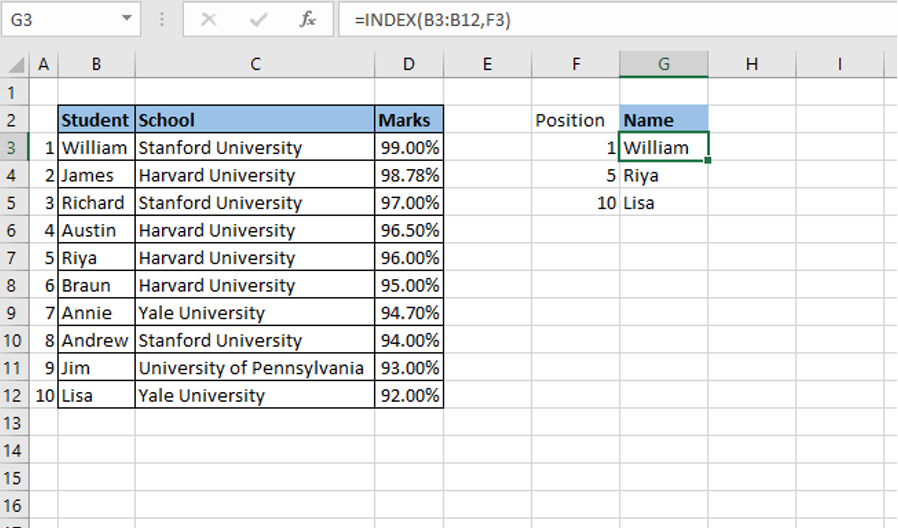
INDEX returns the value in the 1^st, 5^th and 10^th rows of the range.

To make the function more dynamic we have linked the row number with corresponding Position in column F.

What if we want the school name of the students who stood at the 1^st, 5^th and 10^th position with Index Function? In that case, we can select a larger scale from B3 to D12 and give row number of the position (1,5 or 10) and column number of the school (2).

School for:

For 1st position = INDEX(B3:D12,1,2)

For 5th position = INDEX(B3:D12,5,2)

For 10th position = INDEX(B3:D12,10,2)

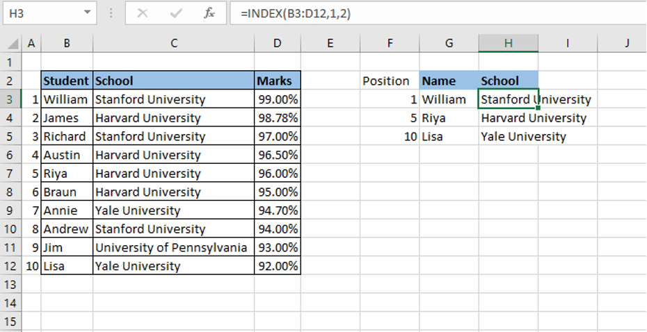
INDEX returns the value at row 1/5/10 and column 2.

In short, we can summarize that INDEX is a dynamic function that gets a value at a given location in an array of cells based on the row and column. If the range is one-dimensional then only row number or column number needs to be updated. However, if the data is two dimensional both row and column number needs to be updated.

However, we often do not know the position of a particular thing in a spreadsheet. For example, if someone wants the position at which Riya is standing amongst 10 students, we will not exactly now where she is standing unless we see the data in the spreadsheet. For this, we can use the Match Function.

MATCH FUNCTION

The Match function in Excel is used to find the position of an item in a range. In short the MATCH function returns the relative position of an item in an array that matches a specified value in a specified order.

The Syntax of Match Function is:

Explanation of each parameter:

• Lookup_value: is the value you use to find the value you want in the array, a number, text or logical value, or a reference to one of these.
• Lookup_array: is a contagious range of cells containing possible lookup values, an array of values, or a reference to an array.
• Match_type: is a number 1,0, or -1 indicating value to return.

1 or omitted – When we want to find the largest value that is less than or equal to the lookup value. The lookup array has to be sorted in ascending order for this.

0 – When we want to find the first value that is exactly equal to the lookup value. In the INDEX / MATCH combination we almost mostly need an exact match. For this we should set the third argument of your MATCH function to 0.

-1 –When we want to find the smallest value that is greater than or equal to lookup_value. The lookup array has to be sorted in the descending order.

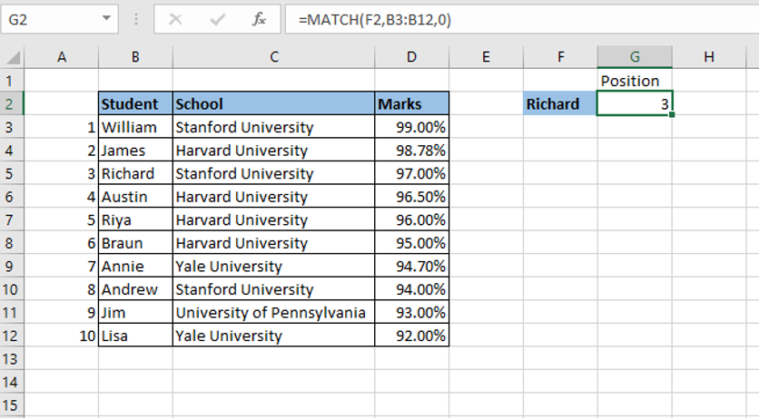
For example, we want to know the position at which Richard is standing amongst the top 10 students in the above example. We can use match function for this as below:

=Match(F2,B3:B12,0)

or, instead we can type the person name in the place of lookup_value.

=Match(“richard”,B2:B12,0)

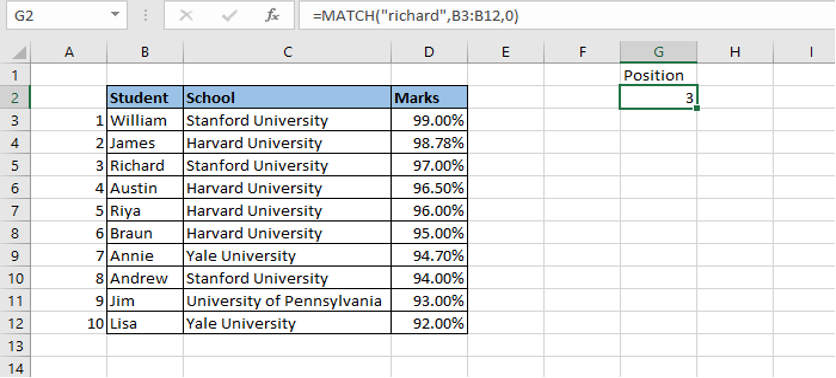
MATCH returns 3, since Richard is standing at the 3^rd position in the state.

Match function is not case sensitive as we can see above.

Match can be used irrespective of whether the range is vertical or horizontal. Example of horizontal array.

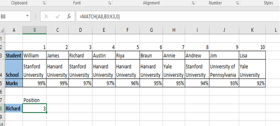
We get the same result with horizontal range, i.e., 3.

INDEX MATCH FUNCTION

In the previous examples we have seen how Index and Match works individually. In Index function we have to input the row and column number. However, in large dataset it is not always possible to know the row or the column number. In this situation, the match function comes to play. The match function can replace the row number, or column number or both in the Index Function. This makes the Index function more dynamic to search or extract any value.

The Syntax of Match Function is:

One-way Lookup

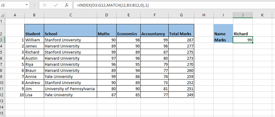
              Modifying the above example, suppose we want the total marks secured by Richard in mathematics. Instead of inputting the row number as 3 in the Index function, we can also use match function.

              Syntax:

             =INDEX(D3:G12, MATCH(J2,B3:B12,0),1)

Two-way lookup             

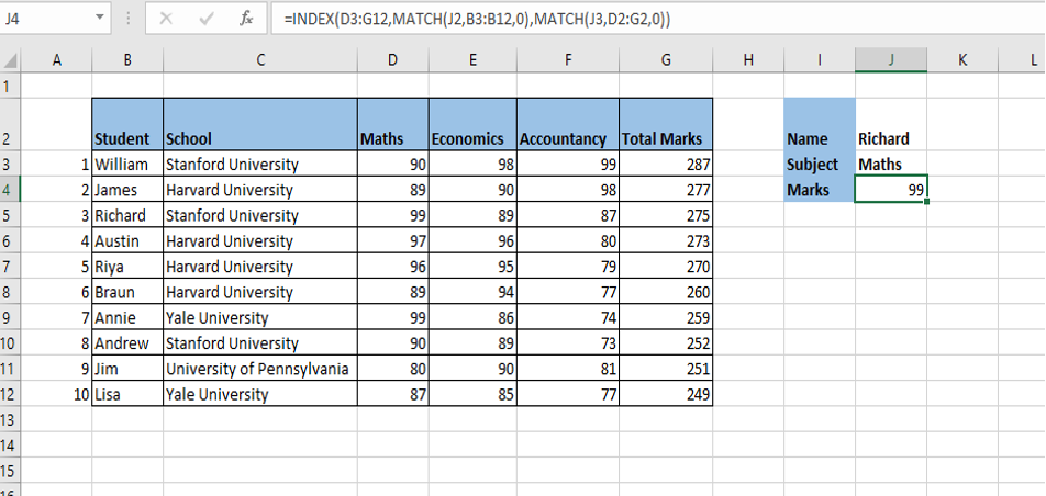
Suppose we want to make the Index function more dynamic, i.e., we want both criteria Name and Subject to be dynamic we can use match function to replace the hard-core row and column number in the Index function.

Taking the sample example above:

Syntax for two dimensional Index Formula:

=INDEX (D3:G12, MATCH (J2, B3:B12,0), MATCH (J3, D2:G2,0))

To Summarize in short:

• The Index function needs a numeric position of row and column
• The Match function helps find those positions
• Match function is nested inside the Index function

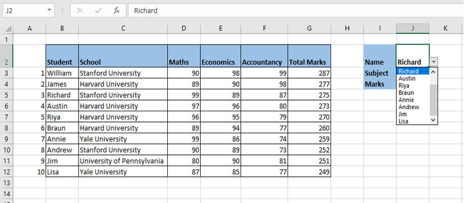
What do we do if we want to find the marks for any other student or we want to find the marks for any other subject? We can use dropdown menus of Name and Subject using data validation.

For Data Validation: Go to the Data tab> then select Data Validation from Data Tools> then select list from Allow box and select the range from the given dataset.

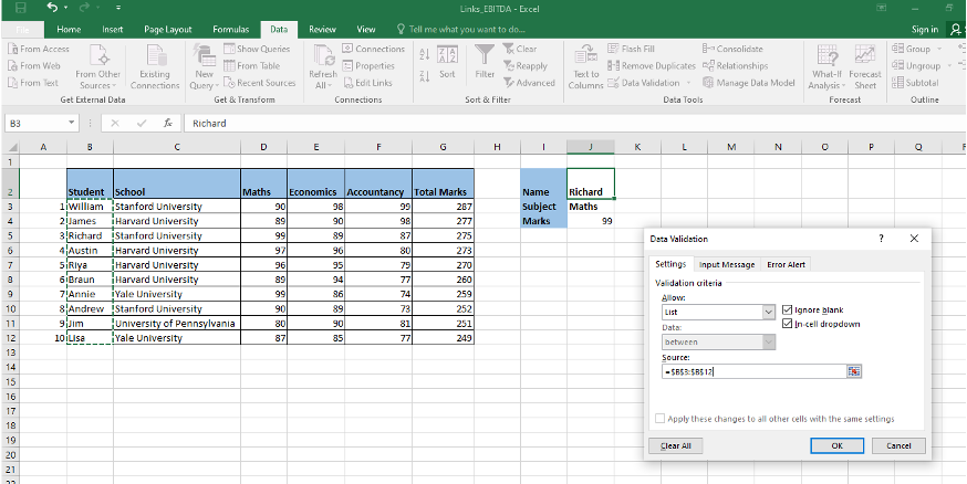
The cell J2 will look like

CASE-SENSITIVE LOOKUP

Though the Index and Match function is not case sensitive, however if we want to lookup values for only case sensitive data, we can use Exact function along with Index and Match function.

Example: We have list of 10 employees with their Employee ID’s. We want employee ID of the employee only for the Name mentioned in the list and in the same case (Upper or Lower).

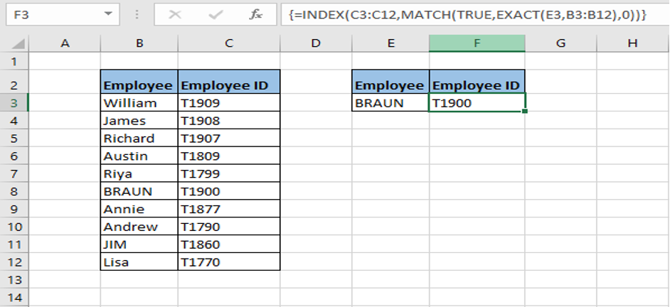
Except in Excel 365, the above formula must be entered as Control+ Shift+ Enter since it is an array formula.

LEFT LOOKUP

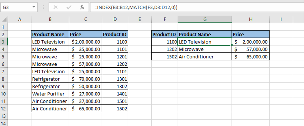
As discussed in the very beginning, Index Match function is better than VLOOKUP function as it can also lookup values to the left unlike VLOOKUP.

Example: We have list of Electronic goods, Price and Product ID. Product ID is given in the last column of the table and we want to retrieve product information based on the Product ID. In this case we cannot use VLOOKUP and have to instead use Index Match function.

CLOSEST MATCH

We can use Index Match function along with MIN function and ABS function to get the closest match to a target in the data column.

Example: We have list of Employee with achieved sales during the year. We have a set target too. Find the Employee who is closest to his or her target.

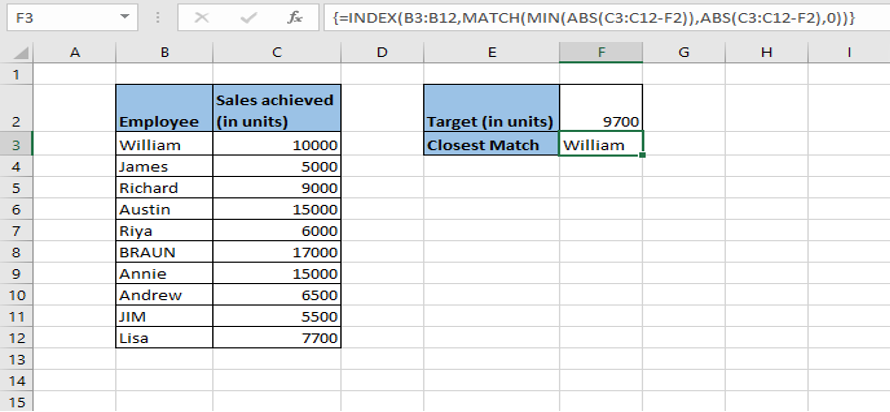
Except in Excel 365, the above formula must be entered as Control+ Shift+ Enter since it is an array formula.

MULTIPLE CRITERIA LOOKUP

Index Match function is perfect to lookup a value based on multiple criteria. Index Match helps to lookup values from one or more than one column at the same time. We can use Index Match with Boolean logic to match 2 to three criteria at the same time.

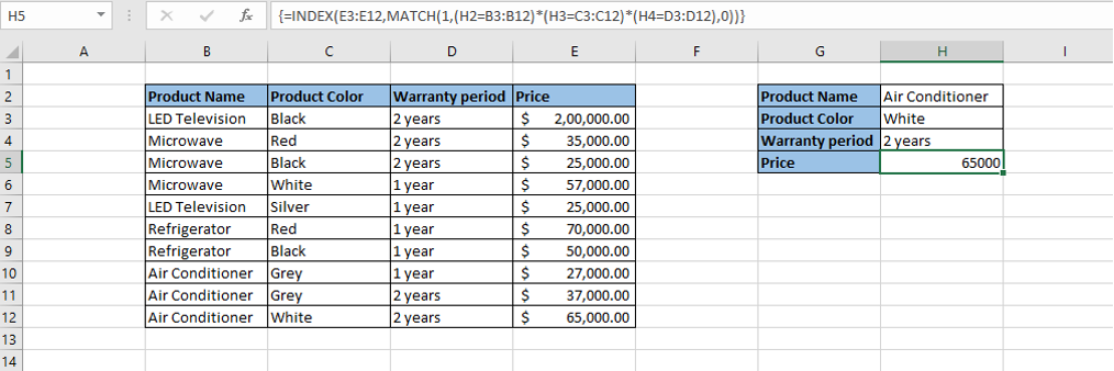
Except in Excel 365, the above formula must be entered as Control+ Shift+ Enter since it is an array formula.

Conclusion:

As you can see with the above illustrations, the Index Match is a very solid Excel function when used in the combination to extract values anywhere in a data set. The fact that data need not be in a very limited way for the VLOOKUP function to work is a very practical and important advantage that Index Match function has. Do carry out the exercises to get a better practice of the use cases for this function.