What is the Transpose function?

The Transpose in Excel function allows you to reorganize your data by flipping it vertically or horizontally. It is a powerful tool that can save you a lot of time and effort when working with large datasets. Instead of manually copying and pasting data, the Transpose function does it for you with just a few clicks.

When to use the Transpose function?

The Transpose function is particularly useful when you want to convert rows into columns or vice versa. For example, if you have a dataset where each row represents a different month and each column represents a different category, you can use the Transpose function to convert it into a dataset where each row represents a different category and each column represents a different month. This can make it easier to analyze and present your data in a meaningful way.

Benefits of using the Transpose function

The Transpose function offers several benefits in Excel. First, it saves you time and effort by automating the process of rearranging your data. Instead of manually copying and pasting, you can simply use the Transpose function to achieve the same result in seconds. Second, it helps you organize your data in a more logical and intuitive way. By converting rows into columns or vice versa, you can make your data easier to understand and analyze.

Finally, the Transpose function enables you to quickly transform your data to suit different reporting or presentation needs. Whether you need to create a chart, a pivot table, or a summary report, the Transpose function can help you achieve your goals efficiently.

How to use the Transpose function in Excel

Using the Transpose in Excel function is easy. Here’s how you can do it:

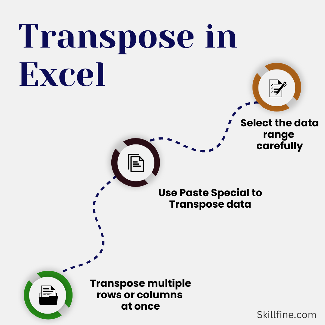
1.       Select the range of cells that you want to transpose.

2.       Right-click on the selected range and choose “Copy” from the context menu.

3.       Select the cell where you want to paste the transposed data.

4.       Right-click on the selected cell and choose “Paste Special” from the context menu.

5.       In the Paste Special dialog box, check the “Transpose” option.

6.       Click “OK” to transpose the data.

Examples of using the Transpose function

Transposing data from a table

Let’s say you have a table in Excel where each row represents a different employee and each column represents a different attribute such as name, age, and department. If you want to convert this table into a format where each row represents a different attribute and each column represents a different employee, you can use the Transpose function. Simply select the range of cells containing the table, copy it, select the destination cell, and choose the “Paste Special” option with the “Transpose” checkbox checked.

Transposing data from a chart

If you have a chart in Excel and you want to convert it into a table format, you can use the Transpose function. Copy the chart, select the destination cell, and choose the “Paste Special” option with the “Transpose” checkbox checked. This will convert the chart into a table format, making it easier to manipulate and analyze the data.

Transposing data from a pivot table

Pivot tables are a powerful feature in Excel that allow you to summarize and analyze large datasets. However, sometimes you may want to rearrange the data from a pivot table to suit your needs. You can use the Transpose function to do this. Simply copy the pivot table, select the destination cell, and choose the “Paste Special” option with the “Transpose” checkbox checked. This will convert the pivot table into a regular table format, allowing you to further manipulate and analyze the data.

Common transpose errors

While the Transpose function is a useful tool, it can sometimes lead to errors if not used correctly. Here are some common transpose errors and how to fix them:

•  #REF! error: This error occurs when the range of cells you are transposing contains references to other cells that are now outside the transposed range. To fix this error, make sure that all the referenced cells are within the transposed range.

•  #VALUE! error: This error occurs when the data you are transposing contains non-numeric values that cannot be transposed. To fix this error, make sure that the data you are transposing only contains numeric values.

•  #NAME? error: This error occurs when you are trying to transpose a formula that contains a named range that is not valid in the transposed range. To fix this error, make sure that all the named ranges used in the formula are valid in the transposed range.

How to fix transpose errors

If you encounter any transpose errors, here are some general steps you can take to fix them:

• Double-check your data: Make sure that the data you are transposing is correct and does not contain any errors or inconsistencies.

• Check your formulas: If you are transposing formulas, make sure that all the referenced cells and named ranges are valid in the transposed range.

• Adjust your ranges: If you are transposing a range of cells that contains references to other cells, make sure that all the referenced cells are within the transposed range.

• Use error handling functions: If you anticipate that your data may contain errors or inconsistencies, you can use error handling functions such as IFERROR or ISERROR to handle them gracefully.

Steps to Transpose Data in Excel

Step 1: Selecting the data range to transpose

Before you can transpose data in excel, you need to select the range of cells that you want to transpose. This can be a single row, a single column, or a range of cells that contain your data. To select the range, click and drag your mouse over the desired cells, or use the keyboard arrow keys to move the cursor to the first cell of your range and then hold down the Shift key while using the arrow keys to extend the selection.

Step 2: Accessing the Transpose in Excel function

Once you have selected the data range, you need to access the Transpose function. To do this, right-click on the selected range and choose the “Copy” option from the context menu. Next, right-click on a blank cell where you want to paste the transposed data and choose the “Paste Special” option. In the Paste Special dialog box, check the “Transpose” box under the Paste section and click on the “OK” button.

Step 3: Applying the Transpose function to the selected data

After accessing the Transpose function, Excel will automatically transpose the selected data and paste it into the desired location. The original data range will remain intact, and a transposed copy will be created. You can now review the transposed data and make any necessary adjustments.

Step 4: Reviewing the transposed data and making any necessary adjustments

It is essential to review the transposed data to ensure that it has been correctly arranged. Check that the rows have become columns, and the columns have become rows. You may need to adjust the formatting, such as column widths and cell styles, to match the rest of your worksheet. Additionally, double-check for any errors or missing data that may have occurred during the transpose process.

Transpose Tips and Best Practices

Avoiding common errors and issues when using the Transpose function

When using the Transpose function, it’s crucial to be aware of some common errors and issues that can arise. One common mistake is not selecting the entire range of data to be transposed. Make sure to include all the necessary cells, as leaving out any data will result in an incomplete transposition. Another issue to watch out for is transposing data that contains formulas. The Transpose function will convert the formulas to their resultant values, so make sure you have the original formulas saved elsewhere if needed.

Handling blank cells or missing data during the transpose process

If your data range contains blank cells or missing data, Excel will transpose them as well. This means that if you have empty cells in your original row, they will become columns in the transposed data. To avoid this, it’s essential to clean up your data before transposing. You can delete the blank cells or fill them with appropriate values. Alternatively, you can use the “Transpose” function in combination with other Excel functions, such as IF or ISBLANK, to handle blank cells or missing data more effectively.

Using keyboard shortcuts for quicker transposing

To speed up the transposing process, you can use keyboard shortcuts in Excel. Instead of right-clicking and selecting options from the context menu, you can use the following shortcuts:

·       Copy: Ctrl + C

·       Paste Special: Ctrl + Alt + V

·       Transpose: E + S + E

By memorizing these shortcuts, you can streamline your workflow and save time when transposing data in Excel.

Combine with other functions

The Transpose function can be combined with other functions in Excel to achieve more complex transformations. For example, you can use the Transpose function together with the INDEX MATCH functions to dynamically rearrange your data based on specific criteria.

Plan ahead

Before using the Transpose function, take some time to plan how you want to rearrange your data. This will help you choose the right range of cells to transpose and avoid any potential errors or inconsistencies.

The limitations of using transpose in Excel

While the Transpose function is a powerful tool, it does have some limitations. Here are a few things to keep in mind:

• Size limitations: The Transpose function works best with relatively small datasets. If you try to transpose a very large range of cells, Excel may become slow or unresponsive.

• Formatting limitations: When you transpose data, Excel does not transpose any formatting applied to the original range of cells. You will need to manually apply formatting to the transposed data if desired.

• Formula limitations: If you transpose a range of cells that contains formulas, Excel does not automatically update the formulas to reflect the new cell references. You will need to manually adjust the formulas if necessary.

The best transpose examples in Excel

Now that you have a good understanding of the Transpose function, let’s look at some of the best examples where it can be applied:

• Converting a row-oriented dataset into a column-oriented dataset: If you have a dataset where each row represents a different record and each column represents a different attribute, you can use the Transpose function to convert it into a dataset where each column represents a different record and each row represents a different attribute. This can be useful when you want to perform calculations or analysis on specific attributes across multiple records.

• Creating a summary report: If you have a large dataset with multiple columns and you want to create a summary report that aggregates the data by a specific attribute, you can use the Transpose function to rearrange the data in a way that makes it easier to create the report. For example, if you have a dataset where each row represents a different product and each column represents a different month, you can use the Transpose function to convert it into a dataset where each row represents a different month and each column represents a different product.

• Rearranging data for charting: If you have a dataset that is not in the right format for creating a chart, you can use the Transpose function to rearrange the data. For example, if you have a dataset where each row represents a different category and each column represents a different month, you can use the Transpose function to convert it into a dataset where each row represents a different month and each column represents a different category. This will make it easier to create a chart that compares the performance of different categories over time.

Advanced applications of the Transpose function

In addition to the basic applications we have discussed so far, the Transpose function can be used in more advanced ways in Excel. Here are a few examples:

Transposing multiple rows and columns in Excel

The Transpose function can be used to transpose not only a single row or column, but also multiple rows or columns at once. To do this, simply select the range of cells you want to transpose, copy it, select the destination cell, and choose the “Paste Special” option with the “Transpose” checkbox checked. This will transpose the selected range of cells.

Transposing data between different worksheets and workbooks

The Transpose function can also be used to transpose data between different worksheets or workbooks in Excel. To do this, open both the source and destination worksheets or workbooks, select the range of cells you want to transpose in the source worksheet or workbook, copy it, select the destination cell in the destination worksheet or workbook, and choose the “Paste Special” option with the “Transpose” checkbox checked. This will transpose the selected range of cells between the different worksheets or workbooks.

Transpose versus other data manipulation techniques in Excel

While the Transpose function is a powerful tool for rearranging data in Excel, it is not the only option available. Depending on your specific needs, other data manipulation techniques may be more suitable. Here are a few alternatives to consider:

• Copy and Paste: If you only need to rearrange a small amount of data, you can simply copy and paste it manually. This may be faster and more convenient than using the Transpose function.

• Power Query: If you are working with large datasets or need to perform more complex transformations, you can use Power Query, a powerful data analysis and transformation tool in Excel. Power Query offers a wide range of data manipulation options and can handle much larger datasets than the Transpose function.

• Pivot Tables: If you need to summarize and analyze your data, you can use pivot tables. Pivot tables allow you to group and aggregate data in a flexible and interactive way. While pivot tables do not directly transpose data, they can provide similar functionality by allowing you to rearrange and summarize data dynamically.

Conclusion and further resources for mastering the Transpose function

The Transpose function in Excel is a valuable tool for reorganizing your data quickly and efficiently. Whether you need to convert rows into columns or vice versa, the Transpose function can help you achieve your goals with just a few clicks. By understanding its benefits, limitations, and best practices, you can make the most of this powerful function in your Excel workflows.

To further enhance your skills and master the Transpose function, consider exploring additional resources such as online tutorials, video courses, and Excel user forums. With practice and experimentation, you will become proficient in using the Transpose function and be able to apply it to a wide range of data manipulation tasks in Excel.

If you want to take your Excel skills to the next level, consider exploring other advanced features and functions such as Power Query, Pivot Tables, and Macros. These tools can further streamline your data analysis and reporting tasks, making you a more efficient and effective Excel user.

Remember, practice makes perfect, so don’t hesitate to experiment with different scenarios and datasets to fully grasp the power and versatility of the Transpose function in Excel.

CTA: Ready to take your Excel skills to the next level? Explore our advanced Excel courses to become a master in data analysis, reporting, and automation. Start your journey today and unlock the full potential of Excel!