Introduction
Information is the largest resource of the 21st century. We are all surrounded by information and data. Organisations must systematise and dispose of essential information for business decisions. For this purpose, companies mainly use Microsoft Excel. Microsoft Excel is a spreadsheet software that enables systematic data arrangement. With MS Excel, businesses can easily manage large databases. Excel has numerous functions and formulas, of which the most frequently used ones are discussed in our Excel Cheatsheet Blog. In this article, we will learn about Match Function in Excel.
What is the Match Function in Excel?
The Excel Match function helps determine the position of a value within a given data set. It returns the position of the value we are searching for in the data set.
The syntax of Match Function:
=MATCH(lookup_value, lookup_array, [match_type])
- lookup_value: It is a required parameter. We use the lookup value to find the value in the data array.
- lookup_array: Lookup array is the data set in which the possible lookup value is present. It is also a required parameter.
- [match_type]: It is an optional parameter, [ ] (Square brackets) denotes that the parameter is optional and can be left.
The match_type specifies how to match the lookup_value with the lookup_array. It has three types.
- 1 – Return the largest value that is less than or equal to the lookup_value. The lookup array must be in ascending order.
- 0 – Returns the value that is equal to the lookup_value. The lookup array must be in any order.
- -1 – Returns the smallest value that is greater than or equal to the lookup_value. The lookup array must be in descending order.
The default value for match_type is 1.
Let’s look over a few instances to see how the Match function works.
Example 1:
Alex the HR manager of XYZ Ltd. He wants to find out the employee ID of the individual who earns a salary of $160,000 annually by using the match function.
Formula =Match(G4,D4:D13,0)

- In cell G4 the lookup_value is the salary of $160,000 per annum.
- D4:D13 highlights the lookup_array of the salary of other employees working in the organisation. In Lookup_array we will find the lookup_value.
- 0 is the match_type that returns the position of the exact lookup_value. When using 0 match_type it is not necessary to arrange the values in ascending or descending order. But when using match_type 1 and -1 the data array must be arranged in ascending and descending order respectively.
Hence, the match function returns the 5th position. The 5th position is held by Employee ID #5 i.e. Rose Simth. So, Rose Smith earns $160,000 annually.
Example 2:
Professor Park took a mock test of 100 marks. The passing score for the mock was 33 marks. With the help of the Match function, she wants to determine how many students scored lower than 33 or failed the test.
We are trying to find a value less than the lookup value of 33 marks. We will use the match type 1 when using the match formula.
For using the Match function with 1 as match type we first have to arrange the data in ascending order.
Formula =Match(F5,C4:C13,1)
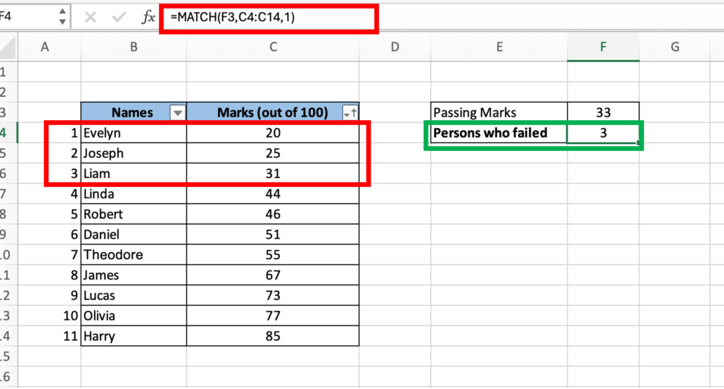
- Cell F3 is for the lookup_value which equals to 33.
- C4:C13 highlights the lookup_array for the marks obtained by the students.
- 1 is the match_type that returns the largest value that is less than or equal to the lookup_value.
The match function has returned the 3rd position, which is the largest value, less than 33 the lookup value. The number 3 represents that there are 3 students who have not been able to secure the passing marks. Note again, it is important that the data is arranged in an ascending order.
Example 3:
Professor Park took a mock test of 100 marks. The passing marks for the mock test were 35%. By using the Excel Match function, she wants to find out how many students have secured higher than the passing marks
Formula =Match(F3,C4:C13,-1)
As we know we are looking for the smallest value which is greater than 35%. So, we will be using -1 in the match type of match function. For this, we have to first arrange the data in descending order and use the Match formula.
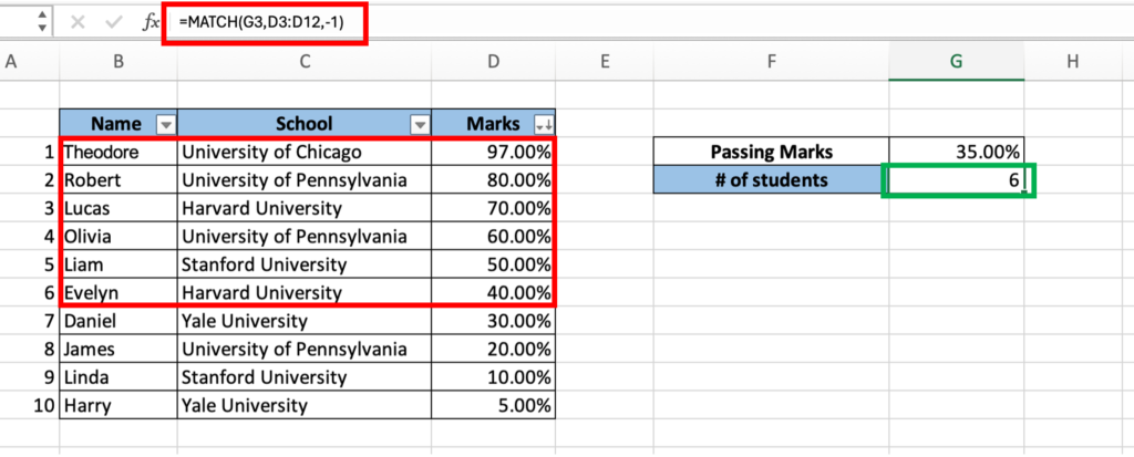
- Cell F3 is the lookup_value of 35% which equals the passing marks for the mock test.
- C4:C13 highlights the lookup_array of the marks obtained by the students.
- -1 is the match_type that returns the smallest value that is greater than or equal to the lookup_value that is 35%.
The match function returns the 6th position. When the data is arranged in descending order, we notice that there are 6 students who have secured the passing marks of above 35%. Notice, in this case the data is arranged in a descending order.
Point to remember for Match Function in Excel:
- The Excel match function is used to find the position of the value within the data set.
- The match function is not a case-sensitive function and does not distinguish between uppercase and lowercase values when matching values from a data array.
- The match function is used to find the exact or approximate match for the lookup value.
- When using match_type 0 it is not necessary to arrange the data array in ascending or descending order.
- When the match_type is 1, the data array must be arranged in ascending order.
- When the match_type is -1, the data set must be in descending order.
- The Match function shows N/A! Error when it fails to find a match for the selected lookup value.