In today’s era, being efficient and productive is significant for a successful career in any field.

In the competitive environment, honing skills that add advantage to your profile helps you bag your dream job. MS Excel is one of these skills. With the help of this Excel Cheat Sheet, you will learn the most valued functions of this prominent program. You can also check out our Excel Course to master one of the most vital skills of the technological era. 

Frequently Used Excel Shortcut Keys:

Some of the Excel shortcut keys that are useful to remember:

1. Ctrl + C: Copy the data.
2. Ctrl + P: Paste the data in the desired cell.
3. ALT + E + S: Special Paste allows to paste formulas, values, etc, in their original format.
4. F2: Used to show & edit the formula within a cell.
5. Ctrl + D: Fill Down
6. Ctrl + R: Fill Right
7. F4: Anchor cells or lock cell reference.
8. Shift + Arrow: Used to select cells.
9. Ctrl + F: Find and Replace.
10. Ctrl + H: Replace Tab.
11. ALT + =: AutoSum. 
12. ALT + I + R: Insert row. 
13. CTRL + – (Minus): To Delete a row/column, first press SHIFT + SPACE: To select the row, press CTRL + – to delete the row.
14. ALT + I + C: Insert column.
15. Ctrl + 1: Opens Format Cell dialogue box.
16. Ctrl + 5: Strick through font.

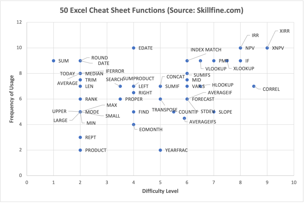
Usage Frequency and Difficulty Levels of Different Excel Functions

We have compiled a list of 50 Excel functions employed by the industry. Let’s now examine the frequency of usage and degree of complexity of these Excel functions.

Range	Difficulty Level	Usage Frequency
1 to 4	Easy	Least Used
5 to 7	Moderate	Moderately Used
8 to 10	Hard	Most Used

We have put together these functions on a 2×2 chart to analyze the ease and frequency of usage of each of the functions to help you priortize some of the functions that you must absolutely know:

We will now to help you understand the syntax of each of these formulas so that you can refer to it as a guide in the future.

Top Excel Cheat Sheet Formulas  

1. =SUM: It adds the series of numbers to give the total.

Syntax: =SUM(number1, [number2], …)

2. =SUMPRODUCT: To calculate the weighted average of a given data set, we use SUMPRODUCT. This function is mostly used to calculate WACC in financial modelling.

Syntax: =SUMPRODUCT(array1, [array2], [array3], …)

3. =AVERAGE: This formula returns the average value of the selected series.

Syntax: =AVERAGE(number1, [number2], …)

4. =MEDIAN: Returns the middle value of the given data set.

Syntax: =MEDIAN(number1, [number2], …)

5. =MODE: Presents the most repetitive value of the data set.

Syntax: =MODE(number1, [number2], …)

6. =PRODUCT: Multiples the value of the selected range of the given data set.

Syntax: =PRODUCT(number1, [number2], …)

7. =MAX: Finds the maximum value in the data set.

Syntax: =MAX(number1, [number2], …)

8. =MIN: Finds the minimum value in the data set.

Syntax: =MIN(number1, [number2], …)

9. =CORREL: Helps to calculate the correlation coefficient between two variables.

Syntax: =CORREL(array1, array2)

• Array 1 represents the independent variables.
• Array 2 represents the dependent variables.

10. =FORECAST: This function is used to forecast future values.

Syntax: =FORECAST(x, known_y’s, known_x’s)

• X value is the value basis on which we want to forecast the values of Y.
• Known_x’s refers to the independent range of data.
• Known_y’s refers to the dependent range of data.

11. =STDEV: The standard deviation function measures the level of dispersion from the mean value in the data set.

Syntax: =STDEV(number1,[number2],…)

12. =VAR.S: The VAR.S function calculates the variance of a sample.

Syntax: =VAR.S(number1,[number2],…)

13. =ROUND: Round function rounds the number to a specified figure of decimal places. 

Syntax: =ROUND(number, num_digits)

• Number is the value we want to round.
• Num_digits are the number of digits to which we want to round the value.

14. =LARGE: Finds the K^th highest value of the given data set.

Syntax: =LARGE(array,k)

• Array: The data which we want to find the largest value.
• k: specifies the largest value which we want from the array.

15. =SMALL: Finds the K^th smallest value of the given data set.

Syntax: =SMALL(array,k)

• Array: The data which we want to find the smallest value.
• k: The smallest value which we want from the array.

16. =LEFT: The LEFT function extracts a character or number of characters from the left side of a text string.

Syntax: =LEFT (text, num_chars)

• Text refers to the string that we want to extract.
• Num_chars refers to the number of characters you want to extract using the left function.

17. =LEN: Len refers to length. It tells the number of characters present in a text string.

Syntax: = LEN(text)

18. =MID: The MID function extracts characters from the middle of a string.

Syntax: = MID(text, start_char, num_chars)

19. =FIND: The FIND formula determines the position of a certain character in a particular data string.

Syntax: =FIND(find_text, within_text,[start_num])

20. =PROPER: The PROPER function is used to capitalise the first alphabet of each word in a data string.

Syntax: =PROPER(text)

21. =REPT: The REPT function repeats the desired text string a certain number of times.

Syntax: =REPT(Text, number_times)

22. =TRIM: The TRIM function removes unwanted spaces between words or characters from a thread.

Syntax: =TRIM(text)

23. =RIGHT: The RIGHT function extracts a character or number of characters from the right side of a text string.

Syntax: =RIGHT (text, num_char))

24. =SEARCH: The SEARCH function searches the position of one text string inside another text string. Unlike the FIND function, the search function is not case-sensitive.

Syntax: =SEARCH(find_text, within_text,[start_num])

25. =UPPER: To convert any lowercase text into uppercase in Excel, the UPPER function is used.

Syntax: =UPPER(Text)

26. =RANK: The RANK function is used to determine the position of a particular value in the given data set.

Syntax: =RANK(number,ref,[order])

• Number represents the value which we want to rank.
• Ref is the series we are referring to.
• Order: If the ranks should be in ascending order or descending order.

27. =IF: The IF function in Excel executes a conditional test to give different results based on the condition.

Syntax: =IF(logical_test, [value_if_true], [value_if_false])

28. =SUMIF: SUMIF is a conditional test which adds the values of the selected cell range meeting the set condition.

Syntax: =SUMIF(range, criteria, [sum_range])

• Range is the data series against which we want to put the criteria.
• Criteria is the condition we are using to determine which values to add.
• Sum_range refers to the data set where the function is applied.

29. =COUNTIF: It is used on a selected range of cells to count the number of cells that meet the condition.

Syntax: =COUNTIF(Range, criteria)

• Range is the data set that we want to count
• Criteria is the condition we put to the test.

30. =AVERAGEIF: AVERAGEIF is a conditional test used for calculating the average value from the selected cell range meeting the set condition.

Syntax: =AVERAGEIF(range, criteria, [average_range])

31. =SUMIFS: The SUMIFS function adds all the arguments in the data set that meet multiple criteria established. It is important to note that the SUMIFS function only works with AND Logic and not with OR Logic.

Syntax: =SUMIFS(sum_range, criteria_range1, criteria1, [criteria_range2, criteria2], …)

• Sum_Range is the series which needs to be added.
• Criteria_range1 refers to the range that is tested for criteria 1.
• Criteria 1 is the first condition.
• Criteria_range2 & criteria 2 refers to the range associated with the second criteria.
• =AVERAGEIFS: The AVERAGEIFS function returns the average of the selected data set that meets multiple criteria.

Syntax: =AVERAGEIFS(average_range, criteria_range1, criteria1, [criteria_range2, criteria2], …)

33. =XLOOKUP: The XLOOKUP function replaces the HLOOKUP and VLOOKUP functions as it is usable for vertical and horizontal data sets. XLOOKUP searches the range of data and returns the first value that matches the corresponding figure.

Syntax: =XLOOKUP(lookup_value, lookup_array, return_array, [if_not_found], [match_mode], [search_mode]) 

• Lookup_value is the value to search for.
• Lookup_array is the data series to search for the value.
• Return_array is the range to return.
• Match_mode specifies the type of match, i.e. exact, smaller number, larger number, etc.
• Search_mode specifies in which mode to perform the search, binary default or reverse.

34. =VLOOKUP: Vertical Lookup searches for the desired value in the first column of the selected data set, and on finding the value, returns the value corresponding to the selected cell.

Syntax: =VLOOKUP(lookup_value, table_array, col_index_num, [range_lookup])

35. =HLOOKUP: Horizontal Lookup looks for the desired value in a horizontal data set (rows). It retrieves the data by searching the top table row, and then returning the value of the corresponding column.

Syntax: =HLOOKUP(value to look up, table area, row number)  

36. =TRANSPOSE: Transpose function flips the selected row into a column and vice versa.

Syntax: =TRANSPOSE(array)

37. =IFERROR: The IFERROR function helps to detect errors in the formula cells.

Syntax: =IFERROR(value,value_if_error)

• Value shows the value to be tested.
• Value_if_Error is the value to be returned if an error occurs.

38. =DATE: The DATE function is used to calculate dates in MS Excel.

Syntax: =DATE(year,month,day)

39. =TODAY: Returns with the current date in the selected cell.

Syntax: =TODAY()

40. =EOMONTH: The End of the month function is used by accountants or finance experts to insert the end date of any month.

Syntax: =EOMONTH(start_date, months)

41. =EDATE: The EDATE function calculates the end date of a period. It is mostly used for debt repayment.

Syntax: =EDATE(start_date, months)

42. =YEARFRAC: Yearfrac calculates the fraction of the year. It is used to calculate stub periods.

Syntax: =YEARFRAC(start_date, end_date, [basis])

• Start Date is the beginning of the period.
• End Date is the end of the period.
• [basis]: Considers the type of day count.

43. =CONCAT: Concatenate Function joins multiple texts from multiple cells into the desired format.

Syntax: CONCAT(string1, string2, …., string_n)

44. =PMT: The PMT functions calculate the constant payments of loan principal and interest figures.

Syntax: =PMT(rate, nper, pv, [fv], [type])

• Rate represents the Interest Rate.
• Nper considers the total number of instalments for loan repayment.
• PV is the present value of the future payments.
• FV is the cash balance left after the last payment.
• Type considers the type of day count that we want to use for the calculation.

45. =NPV: NPV function calculates the Net Present Value for a period of cash flows. NPV function considers all periods as equal. 

Syntax: =NPV(rate,value1,[value2],…)

• Rate represents the discount rate for the period.
• Value 1, and Value 2 represent the payment and income figures.

46. =XNPV: XNPV is an enhanced version of the NPV function. It also calculates the Net Present Value of cash flows for a given period. And it performs calculations with unequal periods.

Syntax: =XNPV(Rate, Cash Flows, Dates of Cash Flow)

• Rate is the discount rate over a period.
• Values are the series of numeric values representing the payments.
• Date shows the dates corresponding to the cash flows.

47. =IRR: It calculates the return for an investment for a series of cash flows.

Syntax: =IRR(values, [guess])

• Value refers to the number for which we want the internal rate of return.

48. =XIRR: Extended IRR is the same as the IRR function, but it values the possibility of irregular periods.

Syntax: =XIRR(values, dates,[guess])

• Values represent the series of cash flows in the worksheet.
• Dates refers to the series of dates of the given value.

49. =SLOPE: This function returns the slope of linear regression based on the given data.

Syntax: =SLOPE(known_y’s, known_x’s)

• known_y’s refers to the array of dependent data sets.
• known_x’s refers to the array of independent data sets.

50. =INDEX MATCH: The INDEX MATCH function is a combination of two Excel formulas:

INDEX: It returns the value based on the data given in the rows and columns of the table.

Syntax: =INDEX(array, row_num, [column_num])

• MATCH: It finds the position of a cell in the row or column of the data table.

Syntax: =MATCH(lookup_value, lookup_array, [match_type])

Conclusion

Excel remains a vital tool for professionals in a variety of industries in this day and age of data-driven decision-making and quickly expanding technology. Its versatility, ease of use, and powerful capabilities make it an indispensable tool for everything from basic data entry to intricate financial modelling and analysis.

Excel empowers users to organise, analyse, and visualise large volumes of data efficiently, enabling them to derive valuable insights and make informed decisions. For financial analysis, forecasting future trends, market analysis and customer demographics, Excel provides a robust platform for conducting sophisticated analyses and driving strategic initiatives.

In conclusion, Excel bridges the gap between traditional spreadsheet analysis and cutting-edge technologies. Its enduring relevance and widespread adoption underscore its importance as a cornerstone of modern business operations, empowering professionals to navigate complex data landscapes. As technology continues to evolve, Excel’s adaptability and versatility will ensure its continued prominence as an indispensable tool for professionals worldwide.