WHAT IS SUMPRODUCT IN EXCEL FUNCTION?

The SUMPRODUCT in Excel function is found under the Math & Trigonometry section of the Formulas Tab in excel. This function not only multiplies the ranges or arrays together and returns the sum of products but also is an incredibly versatile function that can perform sum and count just like the SUMIFS and COUNTIFS function of excel with more flexibility. Other excel functions can also be embedded inside the SUMPRODUCT function that enhances its usage and functionality. SUMPRODUCT is also used to calculate a weighted average. SUMPRODUCT is used widely by financial analysts to handle arrays in different ways and to compare data in two or more than two ranges. Data with multiple criteria can also be calculated using the SUMPRODUCT function.

SYNTAX OF SUMPODUCT IN EXCEL

The syntax of the SUMPRODUCT (array1, [array2], [array3], …)

Where,

• Array1(required argument)- This is the first range or array that we wish to multiply and add subsequently.
• Array2, Array3, … (optional argument)- The second range or array onwards are optional to provide that we wish to multiply and add subsequently.

THE PROPERTIES OF THE SUMPRODUCT IN EXCEL FUNCTION

Some of the important properties of the SUMPRODUCT function are as follows:

1. The minimum number of arrays is 1 in the SUMPRODUCT function were the formula simply adds up all of the array/range elements and returns the sum.
2. The maximum number of arrays that can be used in SUMPRODUCT function is 255 in Excel 2007 to Excel 365 versions while only 30 versions could be used in versions earlier than Excel 2007.
3. Array shortcut is not required in SUMPRODUCT although it works with arrays. We can compete a SUMPRODUCT formula simply by pressing the Enter key.
4. We will get the #VALUE! Error if all the arrays/ranges in a SUMPRODUCT formula do not have the same number of rows and columns.
5. Any non-numeric value contained in an array argument will be treated as zero.
6. We get TRUE and FALSE values if an array is a logical test. We can convert them to 1 and 0 using the double unary operator (–).
7. Wildcard characters are not supported by SUMPRODUCT function.

BASIC USE OF SUMPRODUCT IN EXCEL

Let us understand the SUMPRODUCT function through a simple example.

EXAMPLE: We have Quantity sold and Price of multiple products sold by an Electronics dealer as below. We need to find the total sales made by the dealer.

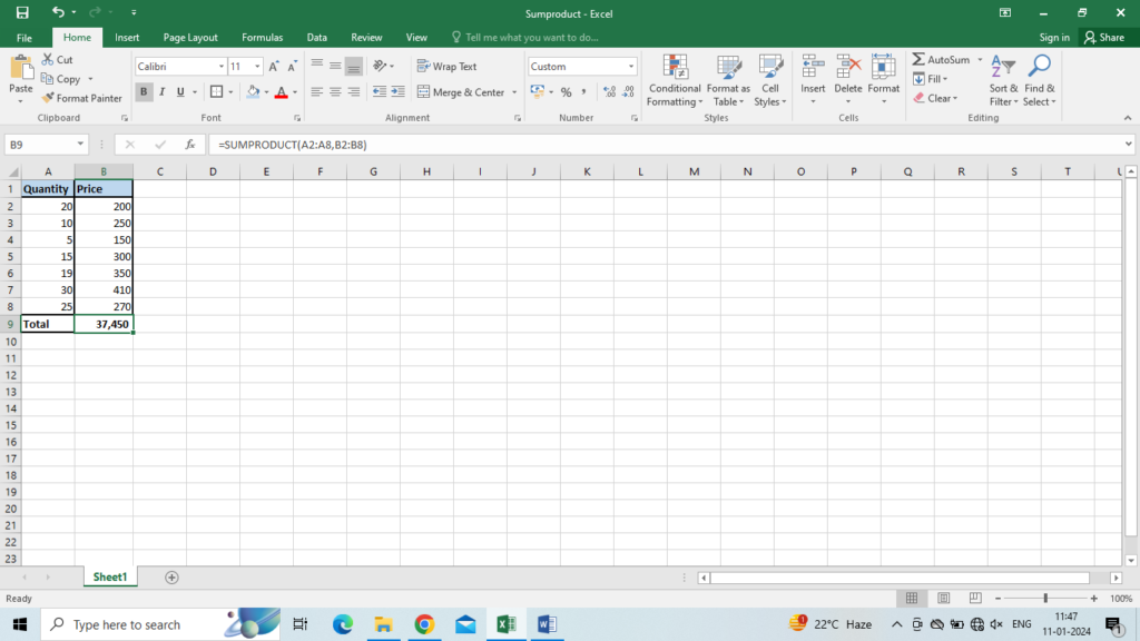
Syntax: =SUMPRODUCT (A2:A8, B2:B8)

A2:A8 represents the first array and B2:B8 represents the second array. At the backend, the SUMPRODUCT function takes the 1^st number in the 1^st array and multiples it by the 1^st number in the 2^nd array and then takes the 2^nd number from the 2^nd array and multiples it with the 2^nd number of the 2^nd array and this continues till the last number of both the arrays. Finally, when all the array numbers are multiplied the SSUMPRODUCT formula adds up the product and returns the sum total.

In short the SUMPRODUCT formula performs the basic simple mathematics as follows:

=A2*B2+ A3*B3+ A4*B4+ A5*B5 ……+A8*B8

SUMPRODUCT IN EXCEL FUNCTION WITH MULTIPLE CRITERIA

The SUMPRODUCT function is used to compare two or more arrays, especially with multiple criteria. Let’s understand this with the help of a simple example.

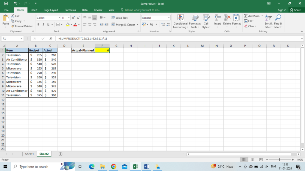
EXAMPLE: ABC Ltd dealing in sales of Electronic Goods have list of some products with its budgeted sales and actual sales figure. ABC Ltd. wants to find how many items have made sales more than the budgeted figure. We can solve this using the SUMPRODUCT function.

Syntax: =SUMPRODUCT (–(C2:C11>B2:B11))

Or,        =SUMPRODUCT ((C2:C11>B2:B11)*1)

Where range C2:C11 is actual sales and B2:B11 is budgeted sales.

If instead of one condition we have more than one condition, we can perform count as follows.

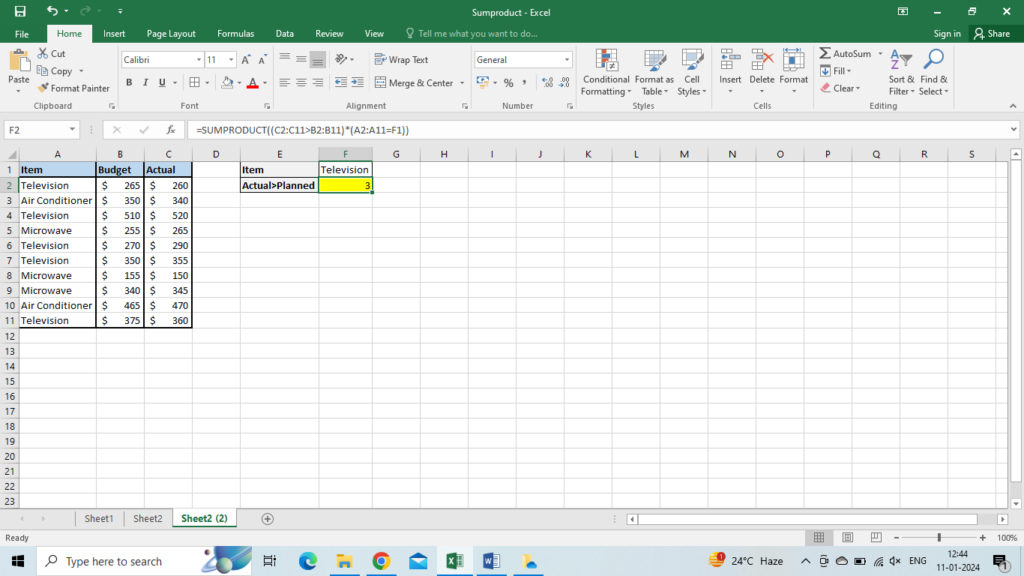
If we want to count how many times Television actual sales is more than budgeted sales, we will add one more criteria to the SUMPRODUCT function.

Syntax: =SUMPRODUCT (–(C2:C11>B2:B11), –(A2:A11=”Television”))

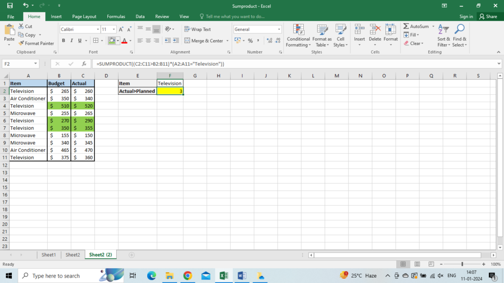
Or,        =SUMPRODUCT((C2:C11>B2:B11)*(A2:A11=”Television”))

Instead of manually writing the product name we can use cell reference as below.

LOGIC BEHIND WORKING OF THE SUMPRODUCT FUNCTION WITH ONE CONDITION

Let’s understand how the SUMPRODUCT function works with 1 condition. From the below screenshot we can see that the Actual sales exceed the budgeted sales approx. by 6 times.

If we select (C2:C11>B2:B11) portion of the formula and press F9, we can see the underlying values of the array as:

=SUMPRODUCT(({FALSE;FALSE;TRUE;TRUE;TRUE;TRUE;FALSE;TRUE;TRUE;FALSE})*1)

We get an array of Boolean values TRUE and FALSE, where TRUE means that the specified condition is met i.e., Actual sales> Budgeted sales and FALSE means that the specified condition is not met i.e., Actual sales< Budgeted sales.

The double negative (–) used in the formulas above is called as double unary operator and it converts the TRUE and FALSE values into ones and zeros. Instead of using double unary operators one can also multiply the array with 1 as in the above screenshot. In both the cases the logical values get converted to ones and zeros as: {0;0;1;1;1;1;0;1;1;0}.

In either case since we have just one array in the SUMPODUCT formula all the 1’s is added to give us the count of actual sales exceeding the budgeted sales. Here we get the count as 6 as there are six 1’s.

LOGIC BEHIND WORKING OF THE SUMPRODUCT FUNCTION WITH MULTIPLE CONDITIONS

When there are two or more arrays in a SUMPRODUCT function, the function multiplies the elements of all the arrays and then adds up the results.

In the example where we found out how many times the Television actual sales exceeded the budgeted sales, we had two arrays with us in the following syntax:

=SUMPRODUCT((C2:C11>B2:B11)*(A2:A11=”Television”))

Or,

=SUMPRODUCT(–(C2:C11>B2:B11),–(A2:A11=”Television”))

Since we have two arrays here, irrespective of whether we use double unary or multiplication operator we get two arrays of ones and zeros. The SUMPRODUCT then functions as normal i.e., it multiplies the corresponding arrays of ones and zeros. Any number multiplied by zero gives zero and hence only if both the arrays have one we will get 1 as a result. Only those rows are finally added to the count that has 1 as a result.

The result works as following in the backend:

SUM/AVERAGE/COUNT CONDITIONALLY OF CELLS WITH MULTIPLE CRITERIA

The feature of SUMIFS, COUNTIFS and AVERAGEIFS was not available in Excel 2003 and older versions

And was introduced only from Excel 2007 version onwards. Till then if one had to conditionally count or sum cells with multiple criteria, one had to resort to the SUMPRODUCT function in Excel. SUMPRODUCT function can work on both AND and/or OR logic in excel. Let’s understand how it works with AND/OR logic through examples.

SUMPRODUCT function with AND logic

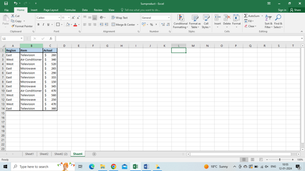
Example: We have a data set of ABC Ltd region wise sales of certain electronic goods and the sales price of each good. We want to get the sum, average and count of sales of Television for the East region.

The SUM, COUNT and AVERAGE though can be solved using SUMIFS, COUNTIFS and AVERAGEIFS functions, we will be solving this using SUMPRODUCT function.

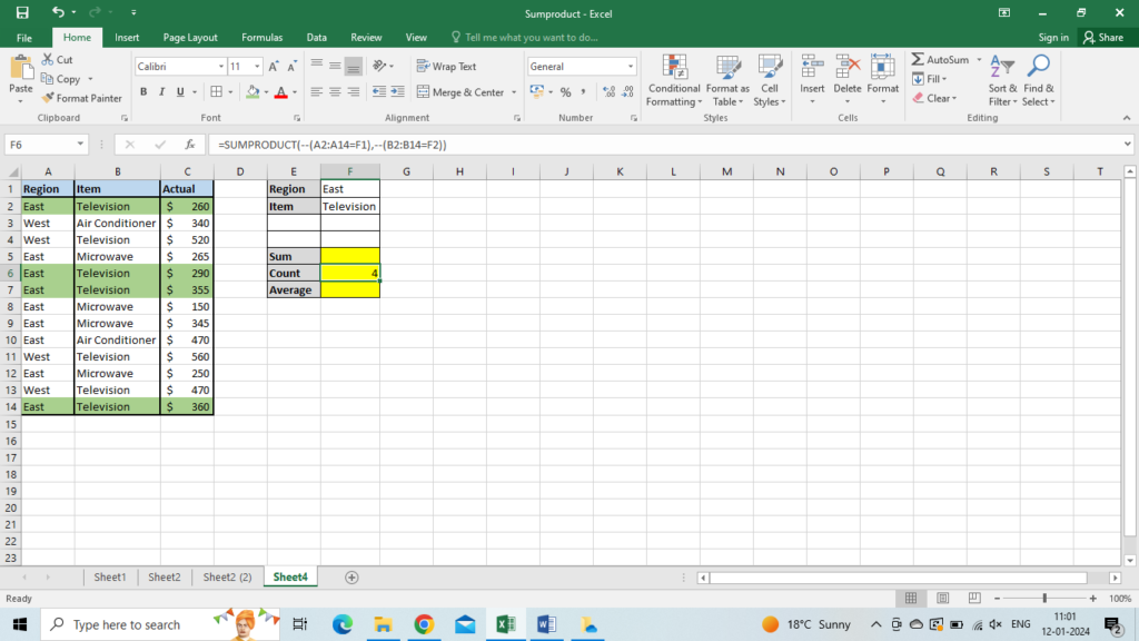
COUNT

To count the Television sales for East region we will use the below syntax:

=SUMPRODUCT(–(A2:A14=F1),–(B2:B14=F2))

Or, =SUMPRODUCT((A2:A14=F1)*(B2:B14=F2))

SUM

To sum the Television sales for East region we will use the below syntax:

=SUMPRODUCT(–(A2:A14=F1),–(B2:B14=F2),C2:C14)

Or, =SUMPRODUCT((A2:A14=F1)*(B2:B14=F2)*C2:C14)

AVERAGE

To average the Television sales for East region we will use the below syntax:

=SUMPRODUCT(–(A2:A14=F1),–(B2:B14=F2),C2:C14)/SUMPRODUCT(–(A2:A14=F1),–(B2:B14=F2))

Logic behind the above conditional sum, average or count

When we use the syntax =SUMPRODUCT(–(A2:A14=F1),–(B2:B14=F2),C2:C14), at the backend we get the following array:

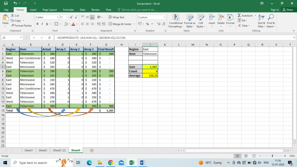
When we multiply the result of array 1, array 2 and array 3, and sum up all the results we get a sum total of $1,265.

SUMPRODUCT function with OR logic

We have to use the plus symbol (+) in between the arrays to conditionally sum or count cells with the OR logic.

In Excel the plus symbol is used in SUMPRODUCT formulas and array formulas to act as OR operator and instructs the excel to return TRUE value if any of the conditions in the formula turns to be TRUE.

For example, if we want to count cells with Television and Microwave sales irrespective of the region we will use the below syntax:

  =SUMPRODUCT((B2:B14=F1)+(B2:B14=F2))

which means count cells is B2:B14=” Television” OR B2:B14=” Microwave”

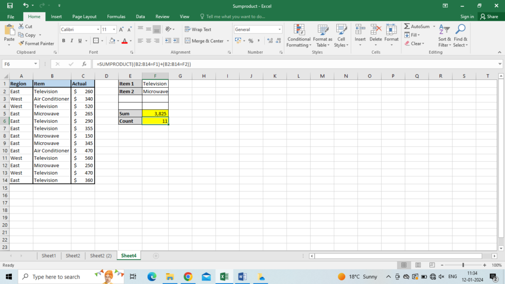
Similarly, if we want the sum of cells with Television and Microwave sales irrespective of the region we will use the below syntax:

=SUMPRODUCT((B2:B14=F1)+(B2:B14=F2),C2:C14)

SUMPRODUCT function with AND as well as OR logic

We can use SUMPRODUCT to get results were we need to use both AND as well as OR logic at the same time.

We can use Asterisk (*) as an AND operator and Plus symbol (+) as an OR operator.

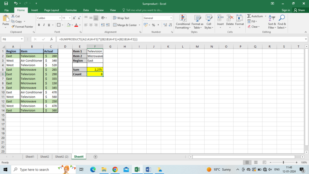
Suppose in the above example, we want to count how many times ABC Ltd. made sales of Television and Microwave in the East Region, we can construct the syntax on the following logic.

=COUNT cells if ( (Region= “East”) AND (Item=”Television”) OR (Item=”Microwave”))

Hence we get the following syntax:

=SUMPRODUCT((A2:A14=F3)*((B2:B14=F1)+(B2:B14=F2)))

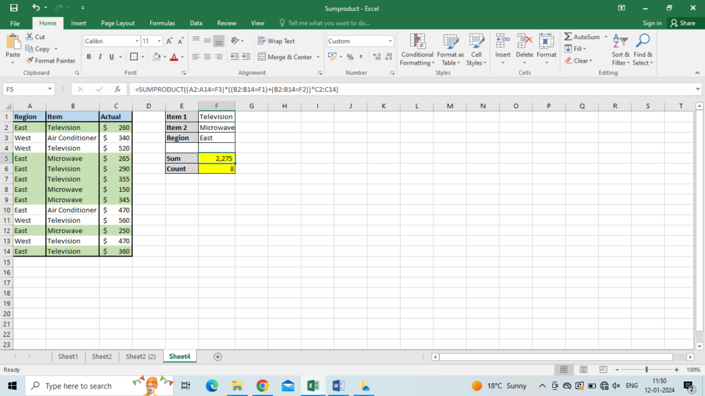
Similarly, to get the sum of Television and Microwave in the East region we will use the below syntax:

=SUMPRODUCT((A2:A14=F3)*((B2:B14=F1)+(B2:B14=F2))*C2:C14)

USING SUMPRODUCT FUNCTION FOR WEIGHTED AVERAGE

The SUMPRODUCT function is used to calculate the weighted average where each value in the range or array is assigned a corresponding weight.

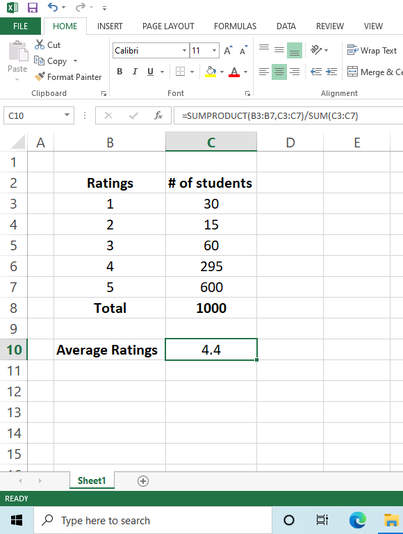
EXAMPLE: Lets say we have the student ratings on a particular program where the students had a choice of entering the reviews on a star ratings scale of 1-5. There were 1000 students in the program and we want to know what was the weighted average feedback on the program.

Syntax: =SUMPRODUCT(B3:B7,C3:C7)/SUM(C3:C7)

As you can see above, the SUMPRODUCT function in Excel is a very useful way to not only do an array multiplication but also have the flexibility to add multiple conditions to the array multiplication if needed. Ideally, you should be able to practice these functionalities on your own so as to be able to do the calculations yourself.

Blog reference: https://www.ablebits.com/office-addins-blog/excel-sumproduct-function/