The COUNTIFS function is a versatile tool and is categorized under Statistical functions in Excel. It is used for counting cells that meet multiple criteria across different ranges. Although both COUNTIF and COUNTIFS functions are used to count cells based on criteria the difference between both the functions is that COUNTIF is used for counting cells with a single condition in one range, whereas COUNTIFS is used to evaluate different criteria in the same or in different ranges.

COUNTIFS helps in doing a quick financial analysis and is used particularly where specific conditional counts are required. For example, it can be used in the Sales analysis where we want to count number of sales above certain criteria in any specific region, attendance tracking where we want to count the number of absentees in a particular month, Inventory management, Inventory management where we want to count no. of inventory of a particular kind below or above a certain inventory level, Survey analysis where we want to count the responses meeting multiple criteria like age, preference of ay product or service or academic performance where we want to calculate number of students who have secured certain marks in any specific subject etc.

The COUNTIFS function is available in all the versions of excel from Excel 2007 to Excel 365. COUNTIFS function counts cells in a single range with a single condition as well as in multiple ranges with multiple conditions and only those cells are counted that meet all of the specified conditions. Each range mentioned in the formula should have the same number of rows and columns as the first range. If any criteria are a reference to an empty cell in excel, the COUNTIFS treats it as a Zero value. Wildcard Characters can be used in criteria like asterisk (*) and question mark (?) and both contiguous and non-contiguous ranges are allowed in COUNTIF function.

COUNTIFS SYNTAX

The syntax used in the COUNTIFS function is as follows:

COUNTIFS (criteria_range1, criteria1, [criteria_range2, criteria2] …)

where,

• criteria_range1 (required)- is the range of cells you want to evaluate for the particular condition. It is used to evaluate the first criteria (criteria 1).
• Criteria 1 (required)- is the condition in the form of a number, expression, or text that defines which cells will be counted. The cells to be counted are defined by the criteria like 5, “<=30”, A7, “Pass”.
• [criteria_range2, criteria2] (optional)- These are additional criteria range and their associated criteria and up to 127 ranges/criteria pairs can be used in the COUNTIF formula.

COUNTING CELLS WITH MULTIPLE CRITERIA

AND LOGIC USED

COUNTIFS function is designed in a way to count only those cells for which all the specified criteria are met and TRUE and works by the AND logic of the AND function in excel.

EXAMPLE 1: Using COUNTIFS function to count with multiple criteria

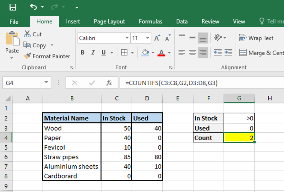
ABC Ltd. has a stock of raw materials and some of which are used in the production of the finished goods. The company wants to find the count of those raw materials that are in stock and is also not used till date, so that the company can consider those raw materials for being re-ordered.

We can use COUNTIFS function to achieve the result as below.

Syntax: =COUNTIFS(C3:C8,G2,D3:D8,G3)

We can make the formula more dynamic by giving cell reference as below

             =COUNTIFS(C3:C8,G2,D3:D8,G3)

EXAMPLE 1: Using COUNTIFS function to count with two identical criteria

We have to input each criteria pair even if the two criteria used in the COUNTIF function are exactly the same.

For example, in the above example we want count of raw materials that are not in stock as well as not used till date.

Syntax: =COUNTIFS (C3:C8, ”=0”, D3:D8, ”=0”)

           Or,

             =COUNTIFS(C3:C8,G2,D3:D8,G3)

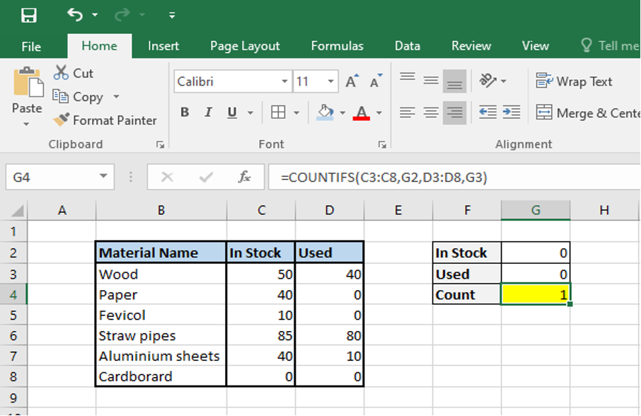
Instead of using multiple criteria in the above example, one may think that a single criteria can be used like =COUNTIFS(C3:D8,”=0”) as both the criteria are same. However, we get a different result as this function typed counts all the zeros from the selected range. We get the following result if we select only one consolidated range.

OR LOGIC USED

The COUNTIF function is designed in a way to return result when all the conditions are specified and based on the AND logic of the AND function in excel as discussed and explained above. However, if we want result based on any one specified condition being true i.e. the OR logic, there are two ways to do this. We can either add up several COUNTIF or COUNTIFS based on the number of conditions to be tested or using the SUM COUNTIFS formula.

EXAMPLE 1: Let us understand how the above OR logic works by adding up the COUNTIF

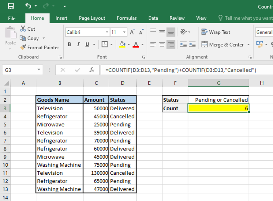
XYZ Ltd sells electronic goods and against each electronic good it has mentioned the status of delivery to the customers as Order Delivered, Pending or Cancelled. ABC Ltd wants to find the count of items that have status as Pending and Cancelled. Let us solve this by adding up the COUNTIF functions.

Syntax: =COUNTIF(D3:D13,”Pending”)+COUNTIF(D3:D13,”Cancelled”)

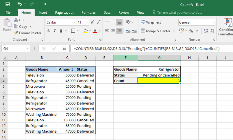
If we want to test more than one condition using the OR logic, we can add up the COUNTIFS function instead of COUNTIF functions.

Suppose in the above electronic goods example, we want to find the count of Refrigerators whose status is Pending and Cancelled. We can add up the COUNTIFS functions to get the desired result.

Syntax: =COUNTIFS(B3:B12,G2,D3:D13,”Pending”)+COUNTIFS(B3:B12,G2,D3:D13,”Cancelled”)

EXAMPLE 2: Let us understand how the above OR logic works by using SUM COUNTIFS function with an array constant.

When we have multiple criteria to check adding up the COUNTIF or COUNTIFS function will not be a viable solution and hence we have an alternative method to find the count using the OR logic instead of adding up the COUNTIF or COUNTIFS functions. A more compact formula exists were we can list all the criteria to be checked in an array constant, and then in the criteria argument of the COUNTIFS function this array can be supplied. We then have to embed the COUNTIFS inside the SUM function to get the total count.

Syntax for the above solution will look like:

SUM(COUNTIFS(range,{“criteria1″,”criteria2″,”criteria3”,…}))

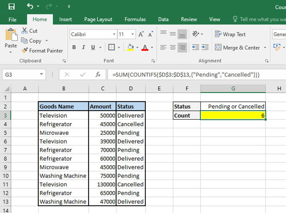
In the above example of electronic goods, if XYZ ltd. wants to find the count of goods that are pending or cancelled, we will use the below syntax.

Syntax: =SUM(COUNTIFS($D$3:$D$13,{“Pending”,”Cancelled”}))

Similarly, if we want to find the count of cells based on two or more criteria pairs, then we need to use multiple criteria pairs within the same COUNTIFS function.

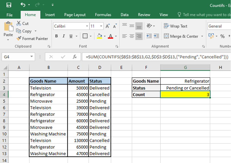
Taking the above example of electronic goods, XYZ Ltd. wants to find the count of Refrigerators that have status as pending OR cancelled, we will use the below syntax.

Syntax: =SUM(COUNTIFS($B$3:$B$13,G2,$D$3:$D$13,{“Pending”,”Cancelled”}))

COUNTING NUMBERS BETWEEN TWO SPECIFIED NUMBERS

Apart from using the COUNTIFS function to count cells based on two or more criteria, we can also use COUNTIFS function to count numbers between any two specified numbers. When we want to find count of cells between any two specified numbers we have to use logical operators like <, >, <= or >=. If we are using logical operators along with the numbers, the same have to be enclosed within double quotes.

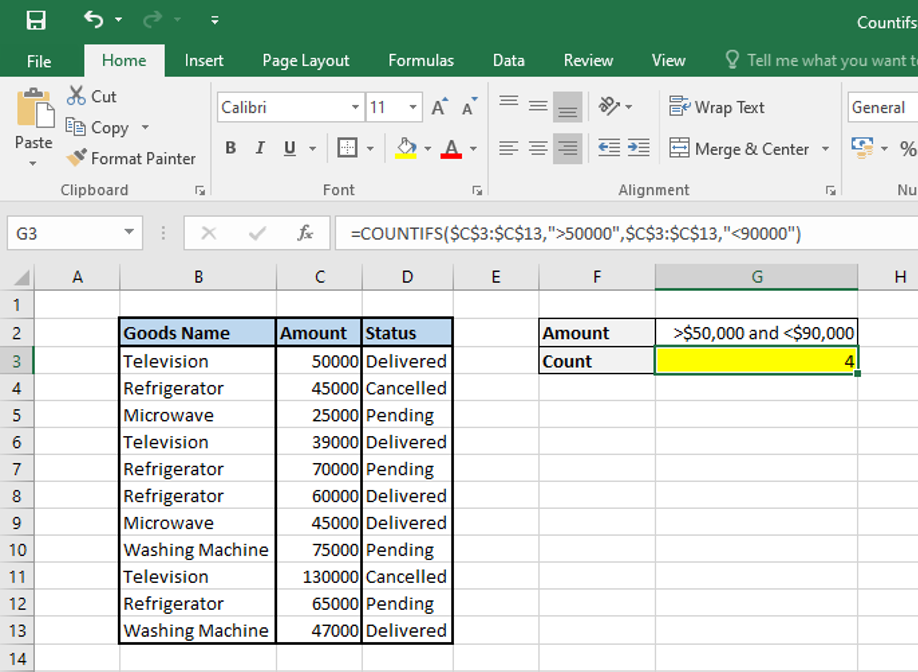
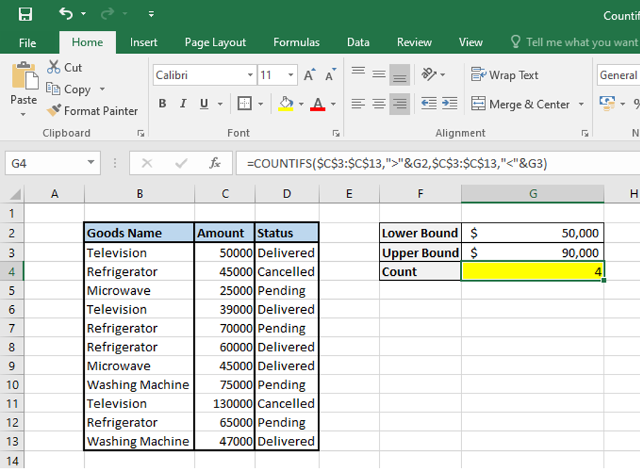
EXAMPLE 1: XYZ Ltd. in the above example of electronic goods want to find the count of goods with value above $50,000 and below $90,000. We will use the below syntax.

Syntax: =COUNTIFS($C$3:$C$13,”>50000″,$C$3:$C$13,”<90000″)

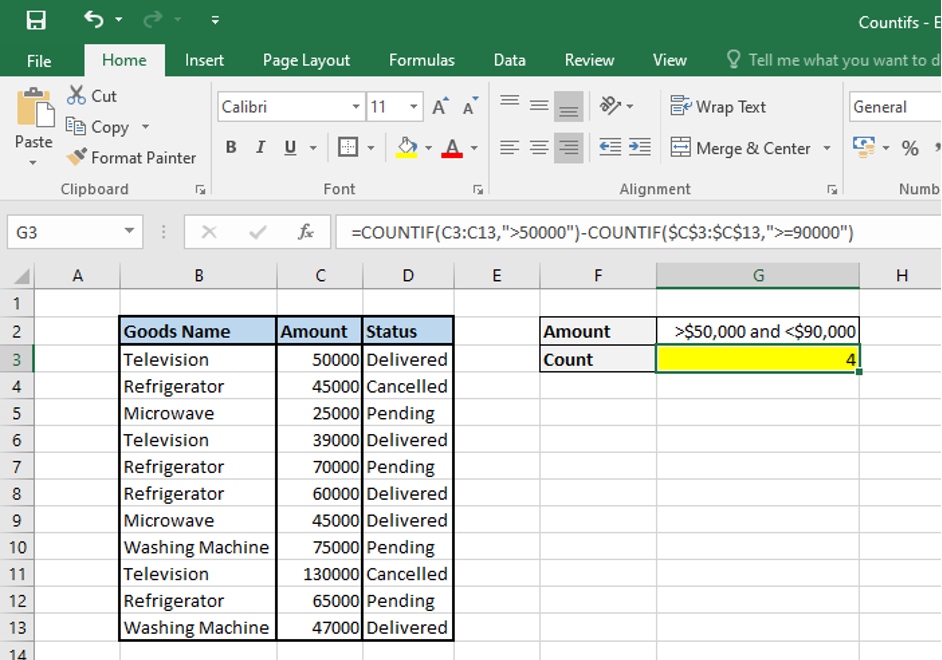
We can also solve the above problem by subtracting one COUNTIF formula from another. The first COUNTIF formula returns the values above the lower bound (i.e. >$50,000) and the second COUNTIF formula returns the values above the upper bound (i.e. >$90,000) and by subtracting the two COUNTIF formulas we get the desired result as above.

Syntax: =COUNTIF(C3:C13,”>50000″)-COUNTIF($C$3:$C$13,”>=90000″)

Point to be noted: In all the above examples if we are using logical operators along with cell references then the logical operator has to be in double quotes and combine the logical operator with the cell reference using the & sign. Let’s explain this using the above example.

Syntax: =COUNTIFS($C$3:$C$13,”>”&G2,$C$3:$C$13,”<“&G3)

USING WILDCARD CHARACTERS IN THE COUNTIFS FUNCTION

We can use the following wildcards in the EXCEL COUNTIFS function:

• Asterisk (*): We can use asterisk to count cells containing a specified word or a character(s) as a part of a cell’s content, since asterisk matches any sequence of characters.
• Question Mark (?): We can use question mark to count cells starting and/or ending with certain characters since question mark matches any single character.

Point to be noted:

• The wildcards only work with text values.
• To match the literal wildcard characters, the tilde (~) character is used. For example, to count cells containing literal question mark (?) we can use “~?” for criteria.
• To count cells that contain text strings that end with a question mark (?). we can add an asterisk (*) sign like “*~?” in the criteria argument.
• Similarly, we can Asterisk (*) with “~*” in the criteria and count tildes (~) with “~~” in the criteria.

EXAMPLE: A college is organising a cultural programme and have listed names of various activities. Against each activity the cultural programme head has to assign a coordinators name and start date and end date each of the activities. All the activities have been assigned the scheduled start date but all the activities have yet not been assigned with the coordinators name and the end date. The cultural head wants to find count of activities that have been assigned with a coordinator name and end date.

Syntax: =COUNTIFS($C$3:$C$11,”*”,$E$3:$E$11,”<>”&””)

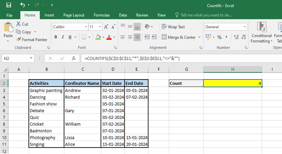
We cannot use the wildcard character in the second criteria since the range contains dates. That why we have to use the character that counts the non-blank cells i.e. “<>”&””.

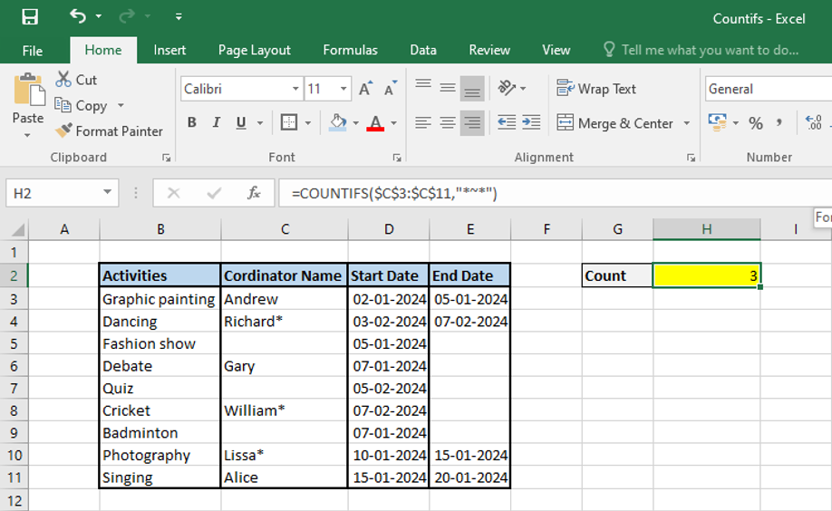
EXAMPLE 2: The cultural head wants to find the count of coordinator names that contains (*) and the end date.

Syntax: =COUNTIFS($C$3:$C$11,”*~*”)

MULTIPLE CRITERIA FOR DATES USING COUNTIFS AND COUNTIF

 EXAMPLE 1: Counting dates in a specified range

Let’s suppose in the above example of cultural programme, the cultural head wants to find the count of activities whose start date is between 5^th Jan 2024 and 31^st Jan 2024.

Syntax: =COUNTIFS($D$3:$D$11,”>=”&DATE(2024,1,5),$D$3:$D$11,”<=”&DATE(2024,1,31))

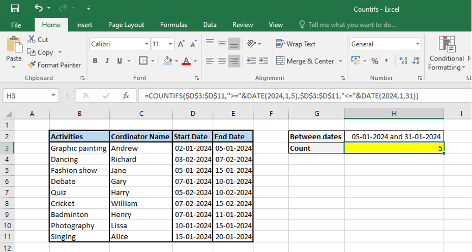
We can also find the solution by subtracting two COUNTIF functions like below.

Syntax: =COUNTIF(D3:D11,”>=”&DATE(2024,1,5))-COUNTIF(D3:D11,”>”&DATE(2024,1,31))

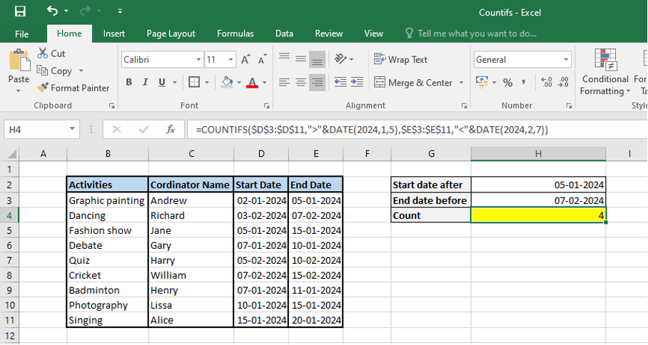
EXAMPLE 2: Counting dates with multiple conditions

Let’s say the cultural head wants to find the count of activities with start date after 5^th Jan 2024 and end date before 7^th Feb 2024.

Syntax: =COUNTIFS($D$3:$D$11,”>”&DATE(2024,1,5),$E$3:$E$11,”<“&DATE(2024,2,7))

Similarly, we can use TODAY () function along with COUNTIFS function.

SUMMARY

We can see from all the above examples that COUNTIFS function is a super dynamic excel function in Excel to count cells based on multiple criteria and can also be clubbed with other excel functions to give us the desired output.