WHAT IS THE SUMIF EXCEL FUNCTION?

SUMIF Excel function is one of the most useful Microsoft Excel function that helps to sum up cells that meet the given criteria. This function is found under Excel Data Tab under the Math and Trigonometry Functions. The criteria can be based on text, number, date, logical operators (such as >, <, <>, =) and also wildcards (such as *, ? ). As a financial analyst or a financial professional we often use SUMIF function since it helps to sum a range of cells based on a given criterion. The best thing about the SUMIF function is that it is supported by all versions of Microsoft Excel.

SYNTAX

The syntax for SUMIF function is as follows:

SUMIF has three arguments, out of which first two are required and the third one is optional.

• Range (required): It is the range of cells you want to evaluate by criteria.
• Criteria (required): is the condition or criteria in the form of a number, expression, date, logical reference or text that defines which cells will be added. It is basically the criteria that must be bet. For example, we can enter criteria like “100”,” Mathematics”,”17/12/2023”, “>100”, “*Delivery*”, etc.
• Sum_range (optional): are the actual cells to be summed if the criteria is met. If omitted, the cells in range are used.

Point to be noted: In the SUMIF function any criteria containing logical operators or any text criteria should be enclosed in double quotations, example: “Delivery”,”>=100”. Any cell reference used in the criteria argument should not be enclosed in double quotation as a result of which they would be treated as text strings.

BASIC SUMIF EXCEL FUNCTION EXAMPLE

Let’s understand the SUMIF function through a simple example.

Suppose ABC Ltd have various stores in different parts of the United states selling various different electronic products. It has maintained an excel data with column B having the Product name, Column C having the region name and column D having the Total Sales figure. ABC Ltd wants to know the sale figure for suppose the North region. We can use SUMIF based conditional addition formula to get the total sales for the North region.

The Arguments in this case would be as follows:

• Range: the list of all regions in column C i.e., (C3:C12)
• Criteria: Cell reference G2 containing the region name or “North”.
• Sum_range: the sales total amount to be added up from column D i.e., (D3:D12)

Syntax:   =SUMIF(C3:C12,”North”,D3:D12)

             Or,

               =SUMIF(C3:C12,G2,D3:D12)

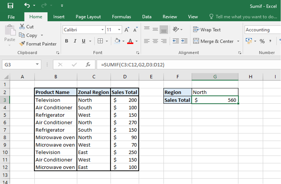
We get the same results from both the syntax used above.

Points to be noted:

1. The SUMIF function is not case-sensitive by nature. Instead of “North” we could have written “NORTH”, ”north” or “nORTH” and we would have got the same result. However, we can force the SUMIF function to sum only case sensitive criteria using Case-sensitive SUMIF function.
2. The Sum_range argument of SUMIF does not necessarily have to be of the same size as the range argument. It means that the sum_range can be of different row or columns from the range argument. For example, the sum_range can D3, or D3:D12 or even D3:D100 and the result will be still correct.

SUMIF FUNCTION WIH LOGICAL OPERATORS

After understanding the basic example of SUMIF function, lets understand SUMIF when used with logical operators combined with text and cell references.

SUMIF function with greater than and less than operator

To get the sum of numbers greater than or less than a particular value, we can use logical operators in SUMIF function. These logical operators can be:

• Greater than (>)
• Less than (<)
• Greater than or equal to (>=)
• Less than or equal to (<=)

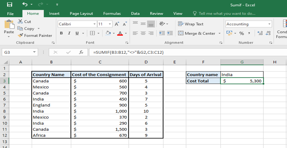
Example: ABC Ltd. Has various consignments of raw materials coming from Different countries and the company wants to arrange funds for the payment of those consignments as and when they arrive. It wants to calculate the total cost of the consignments arriving after 5 days so that it can withdraw the necessary funds from the bank.

Solution: To calculate the total cost of consignment arriving after 5 days we can use the logical operator (>) in SUMIF function along with the text 5 within double quotation or with a cell reference as below:

Syntax: =SUMIF(D3:D12,”>5”,C3:C12)

         Or,

            =SUMIF(D3:D12,”>”&G2,C3:C12)

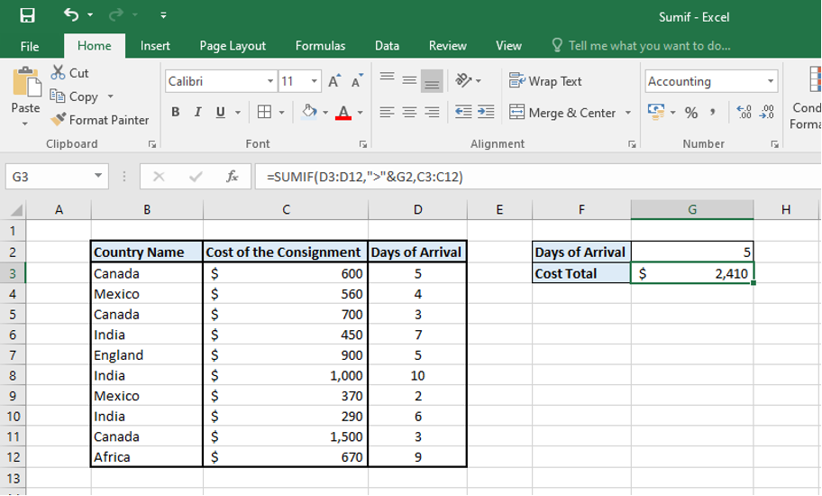
In the above example. If we are using (>) operator before the number, we have to enclose it within double quotation and if we are using the cell reference then we have to enclose the (>) sign only in double quotation and use & sign to concatenate it with the cell reference (G2).

In the similar manner instead of using (>) operator above we can use the other logical operators as the situation demands.

SUMIF Excel function to find equal to

The “equal to” criteria in SUMIF function can be used for both text and numbers and in such criteria the equal to sign (=) is not actually required.

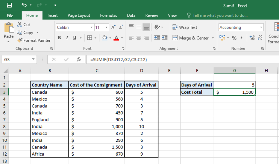
Taking the same example of the consignments above, suppose ABC Ltd. now wants to find the cost of the consignment arriving at exactly at 5 days. In this case we can use the below mentioned syntax.

Syntax: =SUMIF(D3:D12,5,C3:C12) directly the number used

          Or,

             =SUMIF(D3:D12,”=5”,C3:C12)  equal to operator used

          Or,

             =SUMIF(D3:D12,G2,C3:C12)   cell reference used

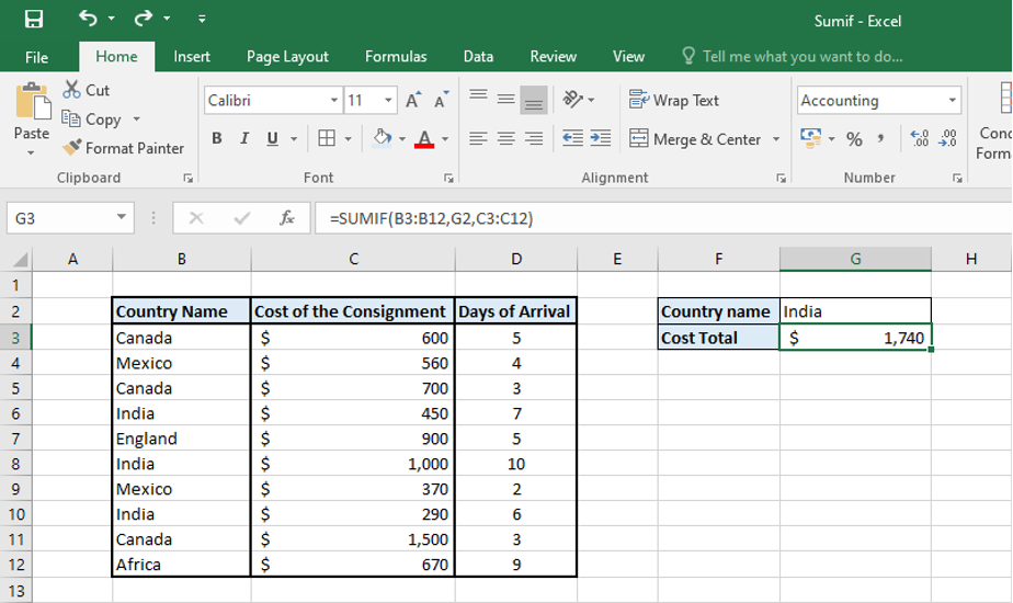
Similarly, we can use the equal to operator with the text values. For example, ABC ltd wants to know the total cost of consignment coming from India, it can use following syntax.

Syntax: =SUMIF(B3:B12, ”India”,C3:C12)

          Or,

              =SUMIF(B3:B12, ”=India”,C3:C12)

          Or,

             =SUMIF(B3:B12, G2,C3:C12)

Points to be notes:

1. In the above example the SUMIF function will add up only the consignment cost from “India” and not from say “North India” or “South India”. To sum up the partial matches, we have to use wildcard characters in the criteria argument of SUMIF function.
2. In SUMIF function any logical operator (>, =>, <, =<, =, <>) whether used on its own or together with a text or number should be always enclosed in double quotation.

SUMIF function to find not equal to

Similar to the equal to operator we can use “not equal to” operator (<>) along with a text or number, and the entire construction should be always enclosed in double quotation If we use the not equal to operator with cell reference then only the not equal to operator should be enclosed within double quotation and then concatenated with the cell reference.

Example: Taking the above example of consignments, ABC ltd wants to find the sum of total cost of consignments coming from all the countries except India. In this case we can use the below syntax.

Syntax: =SUMIF(B3:B12,”<>India”, C3:C12)

             Or,

               =SUMIF(B3:B12,”<>”&G2, C3:C12)

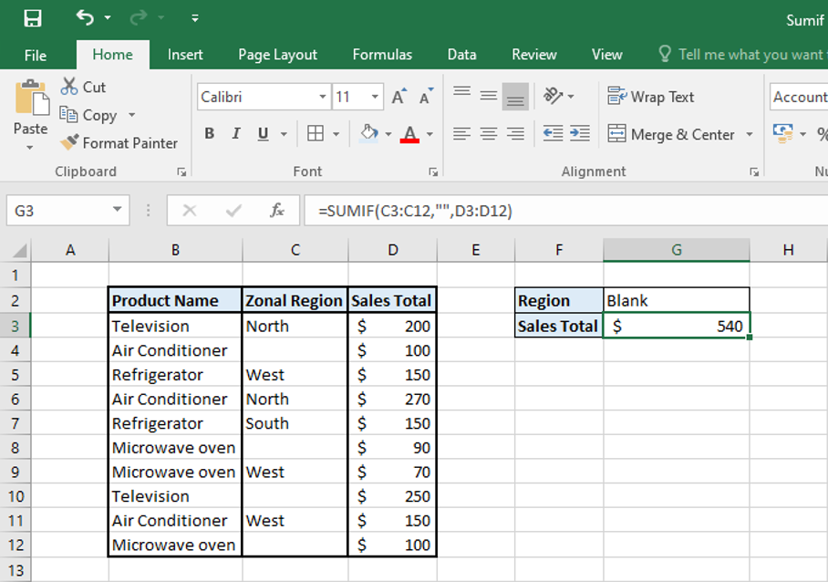
 SUM IF BLANK

We can use the SUMIF function to add up the value of cells in one column for the blank values in another column.

If the blank cell contains absolutely nothing: i.e., no zero length string and no formula we can use “=” for criteria.

If the blank cell contains empty strings: i.e., the cells with formula (=””) then use the “” for criteria.

Example: ABC ltd selling different electronic products in different regions of United States wants to sum up the value of total sales for the Zonal regions not mentioned in the column or where the zonal region is blank.

Syntax: =SUMIF(C3:C12,”=”,D3:D12)

           Or,

              =SUMIF(C3:C12,””,D3:D12)

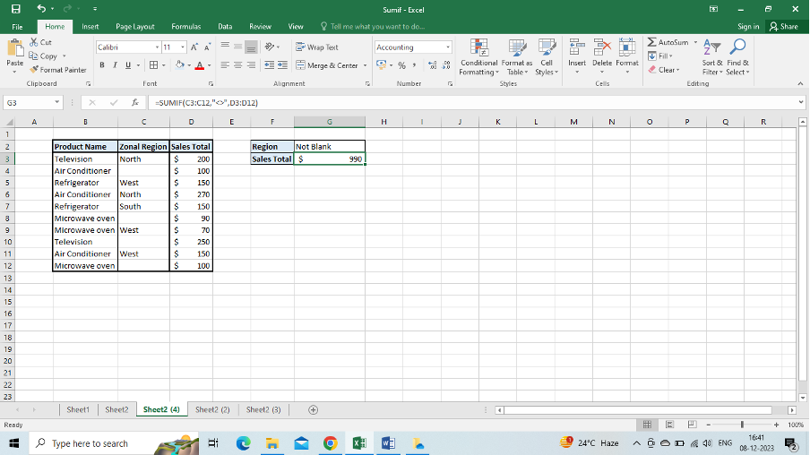
SUMIF NOT BLANK

We can SUMIF function to find the sum of cells where the value is not blank. It also sums up the value of cells containing the zero length string. In such cases we have to use “<>” operator enclosed in double quotation in the criteria argument.

Syntax: =SUMIF(C3:C12,”<>”,D3:D12)

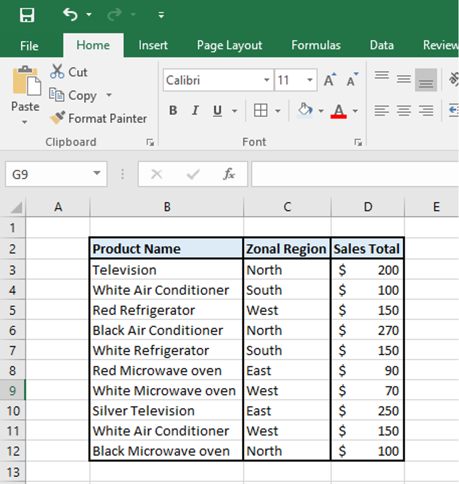
SUMIF WITH DIFFERENT TYPES OF TEXT CRITERIA

SUMIF function can be used to sum up values in one column based on the text values in another column. The sum can be done based on exact match and partial match. We will discuss both cases of exact match and partial match with examples below.

For all the cases to be explained below we are going to take a common example.

Example: ABC Ltd. sells different electronic products of different color and operates in different regions of United States.

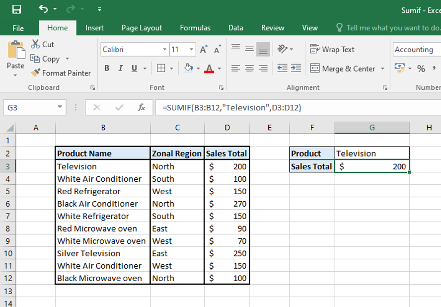
 SUMIF equal to text: Exact Match case

If we want to find the total value of sales for cells containing only the text “Television” we will use the below syntax.

=SUMIF(B3:B12,”Television”, D3:D12)

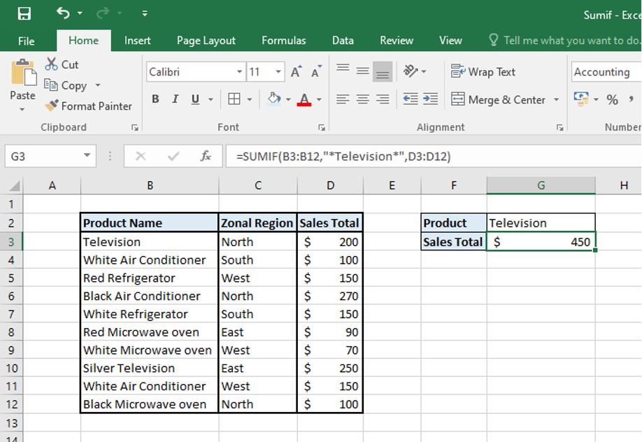
SUMIF if cell contains: Partial Match case

If we want to find the total value of sales for cells containing the text “Television” alone or in combination with other words we will use the below syntax.

=SUMIF(B3:B12,”*Television*”, D3:D12)

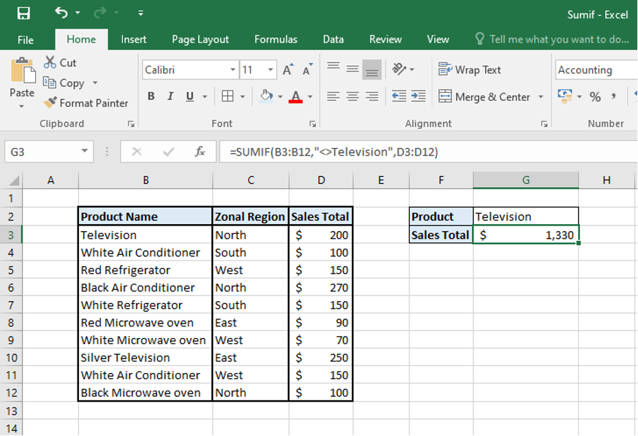
SUMIF if not equal to: Exact Match case

If we want to find the total value of sales for cells not containing the text “Television” alone, we will use the below syntax.

=SUMIF(B3:B12,”<>Television”,D3:D12)

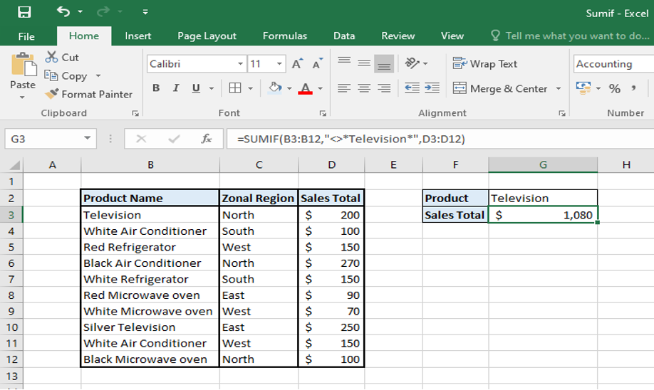
SUMIF if cell does not contain : Partial Match case

If we want to find the total value of sales for cells not containing the text “Television” alone or in combination of other words, we will use the below syntax.

=SUMIF(B3:B12,”<>*Television*”, D3:D12)

SUMIF FORMULAS WITH WILDCARD CHARACTERS

We can use the following wildcard characters in SUMIF formula to sum up cells by partial match:

• to match any number of characters, use Asterisk (*)
•  to match any single character in a specific position, use Question mark (?)

EXAMPLE 1: Sum value of cells based on Partial match

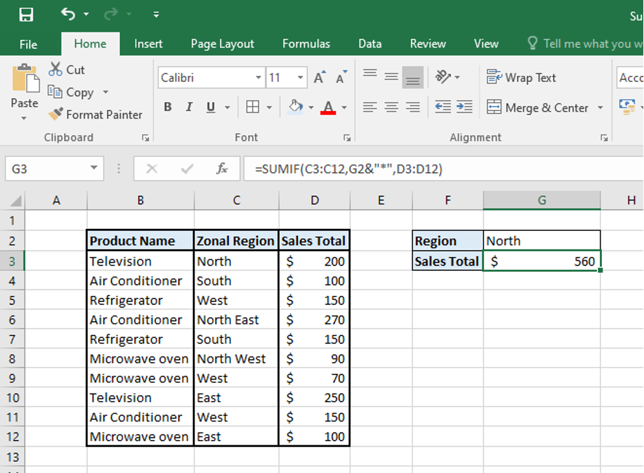
We want to sum the sales of products with regions containing the word North, be it only North, or North west or North east. We can use the following syntax:

=SUMIF(C3:C12, ”North*”,D3:D12)

Or,

=SUMIF(C3:C12, ”*North*”,D3:D12)

Or,

=SUMIF(C3:C12, G2&”*”,D3:D12)

Or,

=SUMIF(C3:C12, ”*”&G2&”*”,D3:D12)

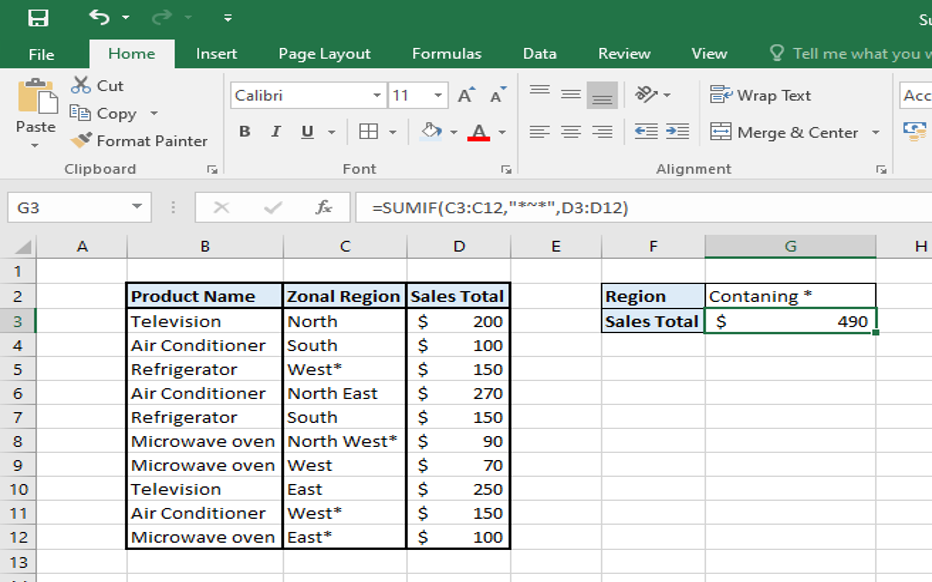
EXAMPLE 2: Sum value of cells if cell contains * or ?

Place a tilde (~) before the * or ? to match an Asterisk or Question mark like “~*” or “~?”.

For example, if we want to find the sales of zones containing the * sign we will use the criteria “*~*”. Here the first Asterisk is the wildcard and the second is a literal asterisk character.

=SUMIF(C3:C12,”*~*”,D3:D12)

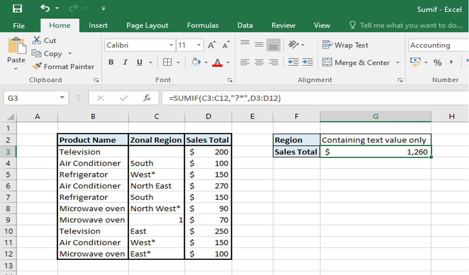
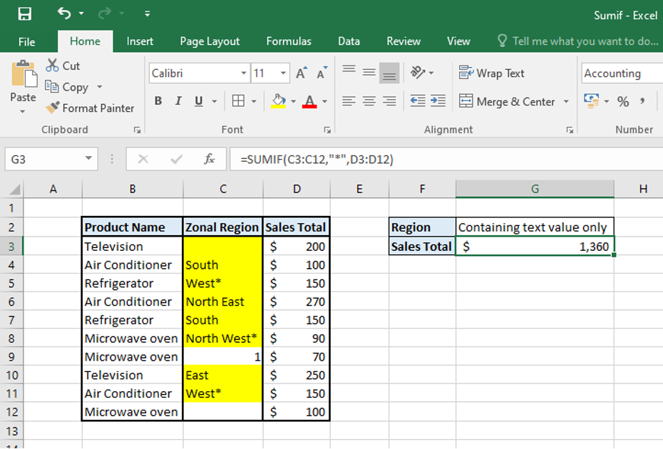
EXAMPLE 3: Sum value of cells that contain any text value ignoring any other type of number, date, error and Booleans

We can use the criteria “?*” if we want to the sum of cells containing only text values ignoring any blank cell or containing any number.

=SUMIF(C3:C12,”?*”,D3:D12)

EXAMPLE 4: Sum value of cells that contain any text value ignoring any other type of number, date, error and Booleans but including the cell with zero string like =””

We can use the criteria “*” if we want to the sum of cells containing only text values ignoring any other type of value but including the cells with zero string.

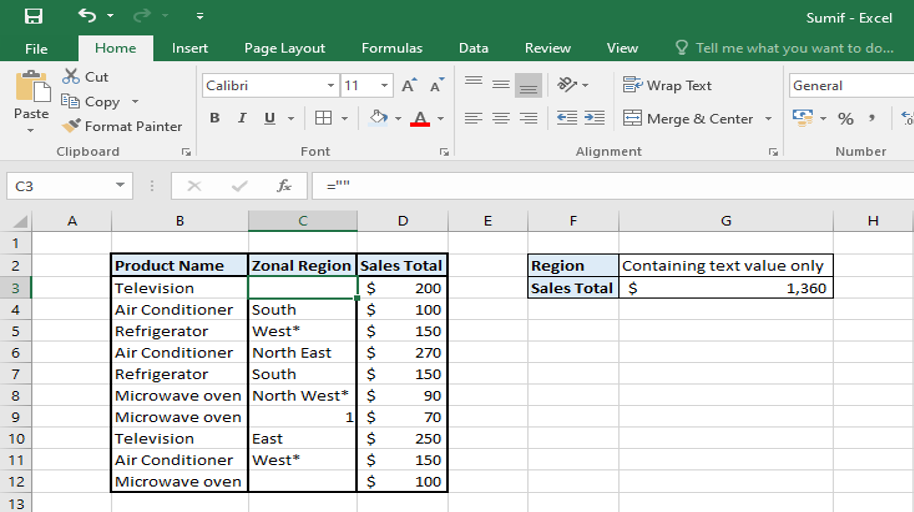
In the above example cell C3 contains zero string =””.

We can use the below syntax to get the result we desire

=SUMIF(C3:C12,”*”,D3:D12)

SUMIF WITH DATE

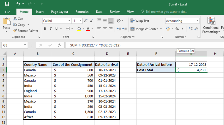
The date can be used like numbers in the SUMIF function, however, the date format should be such that can be understood by excel. We can also use the date function within the SUMIF function as an alternative. We can also use the date as criteria along with logical operators.

EXAMPLE: ABC Ltd has consignments of raw materials coming from different countries on specific dates. ABC Ltd. want to know the total cost of consignment coming on 17/12/2023 or before.

Syntax: =SUMIF(D3:D12,”<=17, C3:C12)

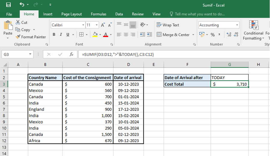
In order to sum based on Todays date, use the TODAY function in the SUMIF function. For example, if we want sum of cost of the consignment later that today’s date, we will use the following syntax:

USING SUMIFS FORMULA FOR MULTIPLE CRITERIA

If we want sum based on multiple criteria, SUMIF function cannot be used. In that case we have to use SUMIFS function. SUMIF calculates the sum of a range based on one or more true or false condition.

SYNTAX: = SUMIFS ( sum_range,criteria_range1,criteria1,criteria_range2,criteria2,…….)

Where,

• Sum_range : are the actual cells to sum
• Criteria_range1: is the range of cells you want evaluated for the particular condition
• Criteria1: is the condition or criteria in the form of a number, expression, or text that defines which cells will be added

Example: ABC ltd wants to calculate the total cost of consignment arriving between the dates 1/12/2023 to 31/12/2023. We will use SUMIFS function here since we are calculating the sum based on more than one criteria.

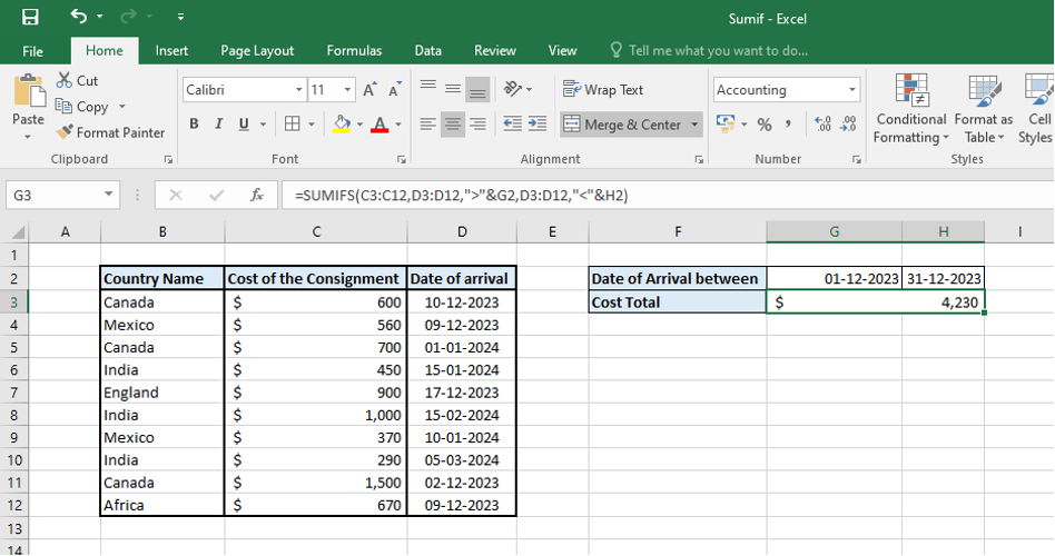
SUMIFS function is a very useful variation of the SUMIF function when we are dealing with multiple conditions to be met before adding up the data in the given analysis.

You can also read this on our LinkedIn company page below: