XLOOKUP is a function which is newly introduced function in MS Office 365. It can be used in place of VLOOKUP as well as HLOOKUP, Index, Match and much more.

Here are a few advantages of using a XLOOKUP function.

• Lookups in both vertical and horizontal ranges
• XLOOKUP does not break when we insert new rows and columns to the data set
• XLOOKUP can help you get the values both from the left as well as the right of the lookup range (better than VLOOKUP). It can help you get values from the Cells above as well as below the lookup range (better than HLOOKUP).
• It can help you find the first as well as last occurrence of a value.
• It does an exact match by default but can also find the nearest number if the exact match is not found.
• It also helps in error handling in case the LOOKUP value is not present in the data source.
• It can return a range of cells or a single cell (as done by INDEX function)
• It also supports wildcards for partial matches.

HAVE YOU CHECK OUR MONTHLY SUBSCRIPTION FOR ALL COURSES, Click here

Let’s understand XLOOKUP function

XLOOKUP Syntax

=XLOOKUP(Lookup_value, lookup_array, return_array, [if_not_found], [match,mode], [search_mode])

The first 3 inputs are compulsory, while the other three are optional.

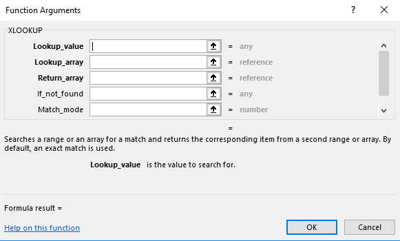
Arguments

Lookup_value – It is the value which we want to search for

Lookup_array – It is the array or range where we want to search

Return_array – It is the array or range we want to be returned by the XLOOKUP function

If_not_found – It is the value to return if the Lookup value is not found.

Match_mode – Here the user has to specify how to match the lookup value against values in lookup array.

• Default value is 0 which means exact match.

Other options available are;

• -1 which means exact match or next smaller one
• 1, means exact match or next larger item
• 2, means wild card character match

Search_mode – Here the user has to specify the search mode to use. By default a first to last search mode is used in the formula.

• 1 is search first to last
• -1 is search last to first
• 2 is Binary search (sorted ascending order)
• -2 is Binary search (sorted descending order)

In this article, we will discuss 2 examples (first two advantages discussed above) and compare XLOOKUP with VLOOKUP and HLOOKUP. We will publish a series of examples over the coming few weeks to highlight the other advantages of using XLOOKUP function.

Avail Data Cleaning and Analytics in Excel for free

Example 1

Comparison with VLOOKUP

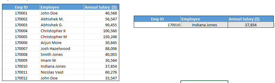
We have a list of employees with their Employee ID and annual salary in the database. See below.

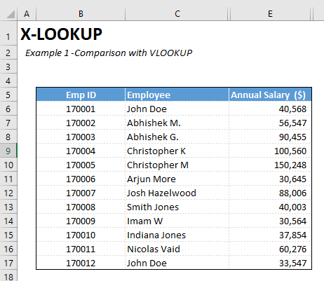
We want to pull the salary of employees in our excel model. How can we do it?

We can use either a VLOOKUP function or XLOOKUP.

Let us discuss how to use XLOOKUP.

For XLOOKUP, we will use just the first 3 variables (Ie; Lookup_value, Lookup_array and return_array).

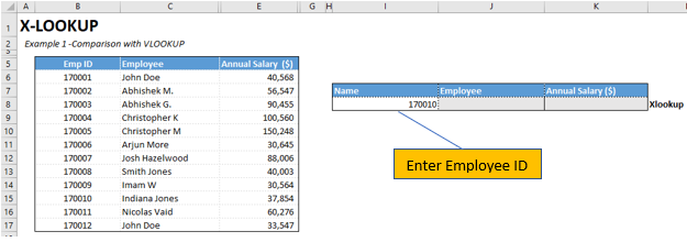
We want to pull the data using the employee ID. Where if we enter the employee ID, we get the employee name and his annual salary.

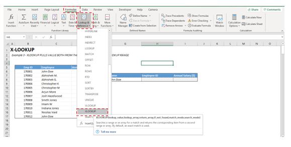
Go to Formulas, Select Lookup & Reference and then Select XLOOKUP.

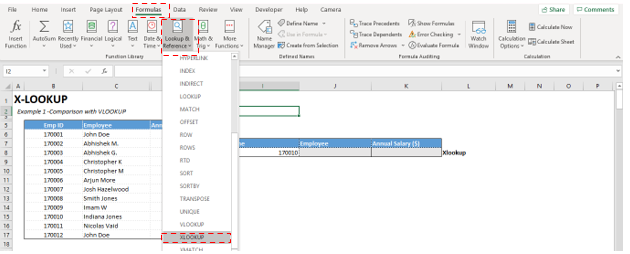
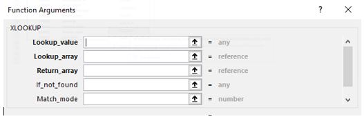
You get the following Function argument.

 

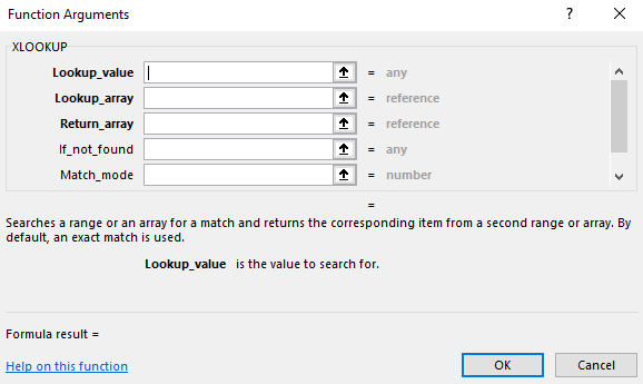
We will start with the employee name.

Lookup_value is the Employee ID. Link it to “Cell I8”

Lookup_array is the Range (B6:B17)

Return_array is the Range (C6:C17)

Leave other function arguments blank and then press OK.

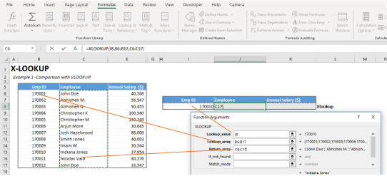
Similarly, for annual salary, the first two selections are the same.

For the Return_array, select the range (E6:E17). Then press OK.

You get the following output.

The advantage of XLOOKUP over VLOOKUP is that on inserting new columns, XLOOKUP keeps working while VLOOKUP loses the output.

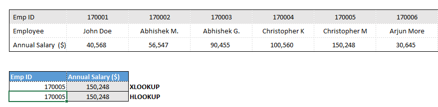
Below Figure shows, output from XLOOKUP and VLOOKUP formula’s

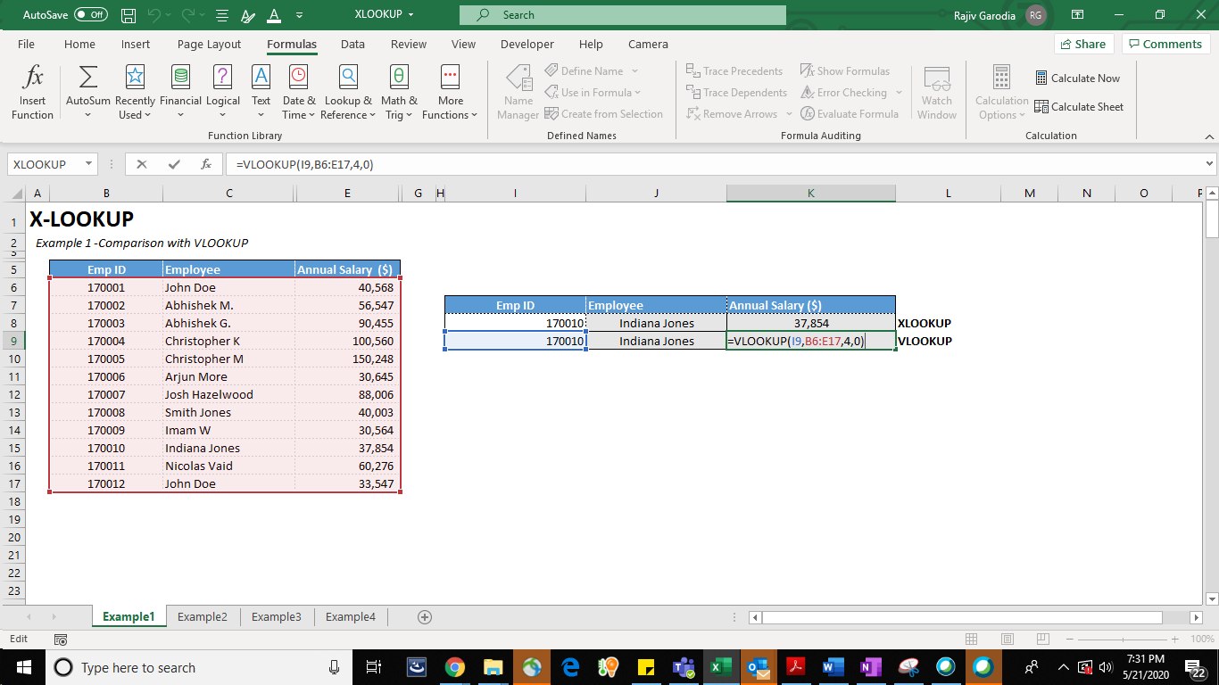
When we insert a column in before column E, this is what happens to the two formulas.

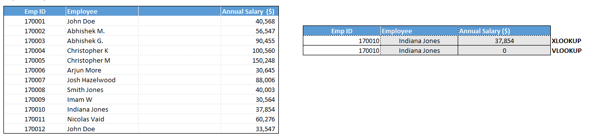
While the annual salary calculated using VLOOKUP function stops working, the new XLOOKUP function is not impacted by the inserted new column.

So, it is advantageous to use XLOOKUP over VLOOKUP function.

Check out how to do data analysis using Pivot Tables.

Example 2

Comparison with HLOOKUP

We have the same data (as in the example above) produced horizontally, see below. We want to pull the annual salary for employees with their EMP ID (as done in the previous example).

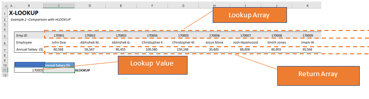
We will start as follows.

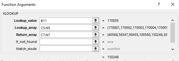
Lookup_value is the Employee ID. Link it to “Cell B11”

Lookup_array is the Range (C5:N5)

Return_array is the Range (C7:N7)

The advantage of XLOOKUP over HLOOKUP is that on inserting new rows, XLOOKUP keeps working while HLOOKUP breaks.

Below Figure shows, output from XLOOKUP and HLOOKUP formula’s

When we insert a column in before row 6, this is what happens to the two formulas.

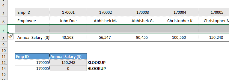
Just as in the case of VLOOKUP, the annual salary calculated using HLOOKUP function stops working, while the new XLOOKUP function is not impacted by the inserted new row.

So it is advantageous to use XLOOKUP over HLOOKUP function.

Still having hiccups in Excel, try our online EXCEL COURSE that comes with live interactive sessions.

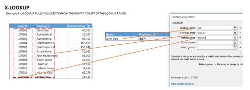
Example 3

PULLS VALUE BOTH FROM THE RIGHT AND LEFT OF THE LOOKUP RANGE

We have a list of employees with their Employee ID and annual salary in the database. See below.

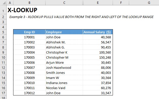
We want to pull the ID and annual salary of employees in our excel model. How can we do it?

We can only pull the Annual salary using VLOOKUP function (since it is on the right of the Lookup value which is the Employee Name) and not the Employee ID (since it is towards the left of the look up value). However, we can use XLOOKUP to pull both the data sets in our excel model.
 

Let us discuss how to use XLOOKUP.

For XLOOKUP, we need to use just the first 3 variables in this example (Ie; Lookup_value, Lookup_array and return_array). Here we have the Employee name as the Lookup value and Employee ID and Annual salary as the output.

Go to Formulas, Select Lookup & Reference and then Select XLOOKUP.

You get the following Function argument.

We will start with the Employee ID.

Lookup_value is the Employee name. Link it to “Cell G8”

Lookup_array is the Range (C6:C17)

Return_array is the Range (B6:B17)

Leave other function arguments blank and then press OK.

Similarly, for annual salary, the first two selections are the same.

For the Return_array, select the range (E6:E17). Then press OK.

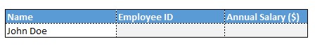
You get the following output.

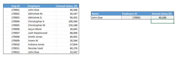
The advantage of using XLOOKUP is that it can pull data both from the left and right columns of the lookup, which was not possible with the VLOOKUP function.

Similarly, XLOOKUP can pull data from rows above and below the LOOKUP array which could not be done using HLOOKUP function.

You can try it by transposing the same example in another excel sheet. Let us know in case you find any difficulty.

Example 4

XLOOKUP FINDS BOTH THE FIRST AND LAST OCCURANCE OF A VALUE

Here is the data showing Customer ID, Name, Date of sale and Amount ($). Name of a few customers is repetitive (Eg. John Doe, Imam W etc.)

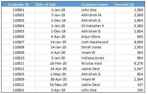
We want to pull the date of last sale and the Sale amount for a few customers.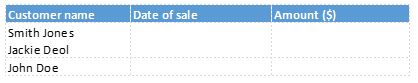

While Smith Jones is appearing just once, Jackie and John are appearing multiple times in the original data. The default value pulled by the XLOOKUP function is the first occurrence, but we have the option to select the Last occurrence when we have multiple entries for the same lookup value.

Here is how we can do it.

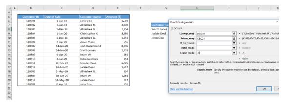
Lookup_value is the Customer Name. Link it to “Cell G8”

Lookup_array is the Range ($D$6:$D$21) , ie; Customer name

Return_array is the Range ($C$6:$C$21), ie; Date of sale

If_not_found – Leave blank

Match_mode – Leave blank

Search Mode – Type -1, as we are finding the last value in the lookup range. Then Press OK.

Fix the Lookup array and return array using F4 key.

Copy and paste the formula in remaining two rows.

Similarly work on the XLOOKUP function for the last sale. First two function arguments are the same. For Return array select range ($E$6:$E$21), ie, Sale Amount.

Search_Mode – Type -1 as we are finding the last value in the lookup range. Then Press OK.

You get the following output.

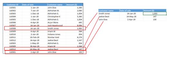
For Smith Jones, we get the Date of Sale as 14 Jan 2020, which matches with the one record present for the customer.

For the other two customers Jackie Deol and John Doe, we get the date of sale as 14^th May 2020 and 2^nd April 2019, which is the last entry in the data range for these customers.

This output was not feasible with any of the other lookup functions, like VLOOKUP, HLOOKUP, INDEX, MATCH or OFFSET function earlier.

Example 5

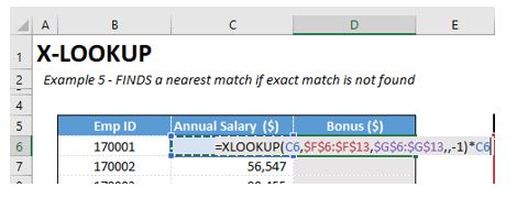
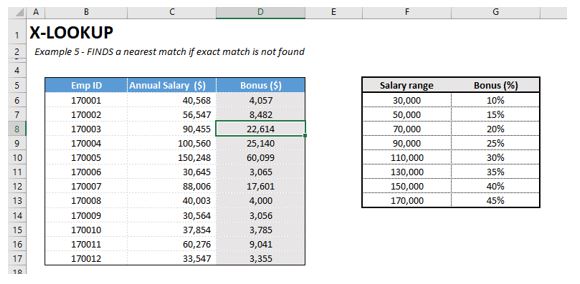
FINDS a nearest match if exact match is not found

We have a data set showing Employee ID and their Annual salary. We also have the % bonus payable for different salary ranges.

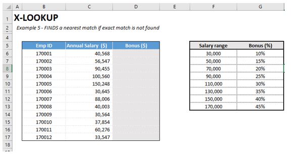
We have to calculate the annual bonus for each employee in column D. Can we do it with one formula?

Yes, it is possible now with X-LOOKUP.

Go to Formulas, Select Lookup & Reference and then Select XLOOKUP.

Enter the following details in the function arguments.

Lookup_value is the Employee Salary. Link it to “Cell C6”

Lookup_array is the Salary Range in the second table (F6:F13)

Return_array is the Bonus Percent Range (G6:G13)

Fix the ranges F6:F13 and G6:G13 using F4 function key

Leave other function arguments blank and then press OK.

You get the following error.

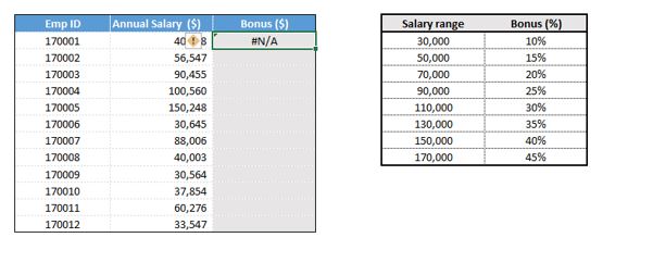
This is because XLOOKUP matches exact value by default. We do not have the exact salary ranges for bonus calculations.

Here, we will have to put an extra argument, as we do not have the exact match for salaries.

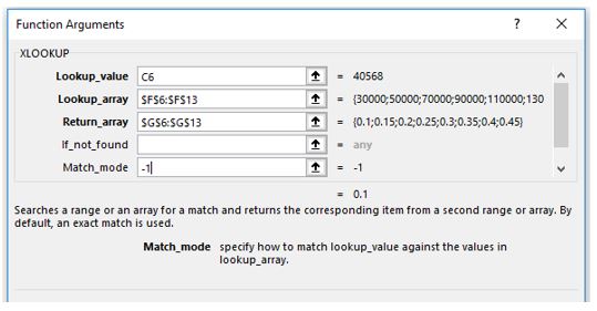
In Match mode enter -1 (instead of leaving it blank or entering 0).

-1 means next smaller value if exact match is not found.

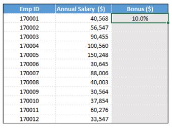
XLOOKUP takes the next lower salary range if exact match is not found. For salary range of $30,000-49,999 the bonus is 10%. Now you get the following output.

In case you want to enter the next larger value enter 1 (instead of -1).

Multiply the Bonus percent with Annual Salary to get the annual bonus.
 

Now copy (Control & C) and paste (Control and V) the formula to calculate bonus for other employees.

Here is the bonus calculation for all the employees.

XLOOKUP has made it easier for us to do complex calculations. In the absence of this function, we would have to place a multiple conditional formula to calculate the bonus in the above example

 

Example 6

HANDLES ERRORS IN CASE THE LOOKUP VALUE IS NOT PRESENT IN THE SOURCE DATA

Here is the data set showing employee ID, Annual salary and Bonus percent.

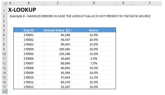
We want to pull the annual salary of few employees in our model.

We can pull the salary nos. using both VLOOKUP and XLOOKUP functions.
 

Let us discuss how to use XLOOKUP.

As discussed in our previous examples, we will use the first 3 variables (Ie; Lookup_value, Lookup_array and return_array). Here we have the Employee ID as the Lookup value and Annual salary as the output.

Go to Formulas, Select Lookup & Reference and then Select XLOOKUP.

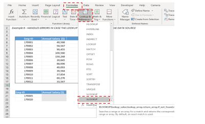
You get the following Function argument.

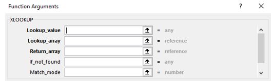
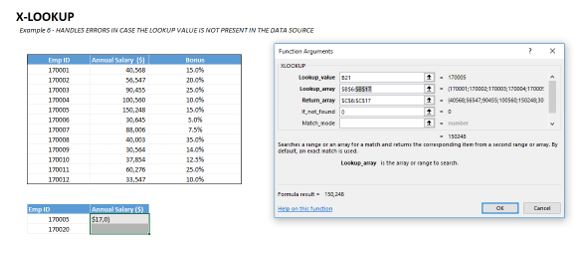
Lookup_value is the Employee ID. Link it to “Cell B21”

Lookup_array is the Range (B6:B17)

Return_array is the Range (C6:C17)

Fix the ranges B6:B17 and C6:C17 using F4 function key

Leave other function arguments blank and then press OK.

You get the following output.

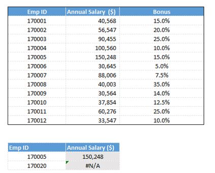
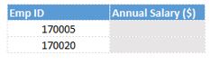
The XLOOKUP function gives us the annual salary for the first employee and not the second. This is because the second employee is not in the original data set as he was not on the payroll during the period of analysis.

To overcome such a situation, we have a function argument IF_NOT_FOUND inbuilt in the XLOOKUP function. Since employee 170020 is not present in the dataset we can use the fourth function argument IF_NOT_FOUND to avoid getting #N/A error.

We will redo the XLOOKUP function.

Now we put a 0 in the if_Not_Found argument and press OK. This time we get the output as shown below.

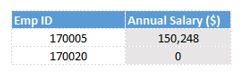
In this case XLOOKUP shows annual salary of the second employee as 0 as he is not in the original data set.
 

If we use a VlOOKUP or index and match here, we will have to use an conditional formula that if the employee is not found put a zero. But it is much easier to put the same condition using a XLOOKUP function.

Example 7

XLOOKUP CAN RETURN A RANGE OF CELLS

This is a very important advantage of using the XLOOKUP function. This feature can help us calculate results for large data sets quite easily.

Let us discuss with the help of an example.

We have daily Sales figures of XYZ Limited from 1^st Jan 2016 to 29^th May 2020. The Data extends till row 1088.

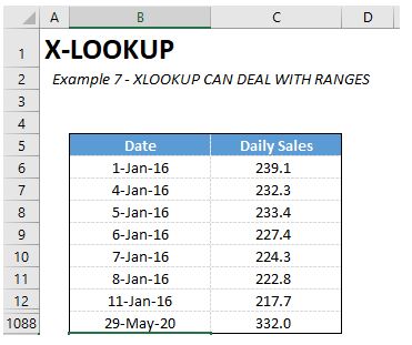
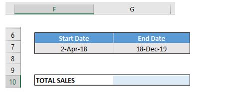
We want to calculate total sales for the Company during selected period.

We can calculate the total sales for selected period easily by using the XLOOKUP Function.

Go to Formulas, Select Lookup & Reference and then Select XLOOKUP.

Enter the following details in the function arguments.

Lookup_value is the Start Date. Link it to “Cell F7”

Lookup_array is the Date Range in the second table (B6:B1088)

Return_array is the Daily Sales (C6:C1088)

Fix the ranges B6:B1088 and C6:C1088 using F4 function key.

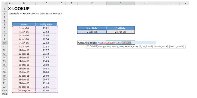
See below, how we can type this formula without going to the FORMULA TAB (as mentioned above)

Leave other function arguments blank and then press OK.

You get the following output

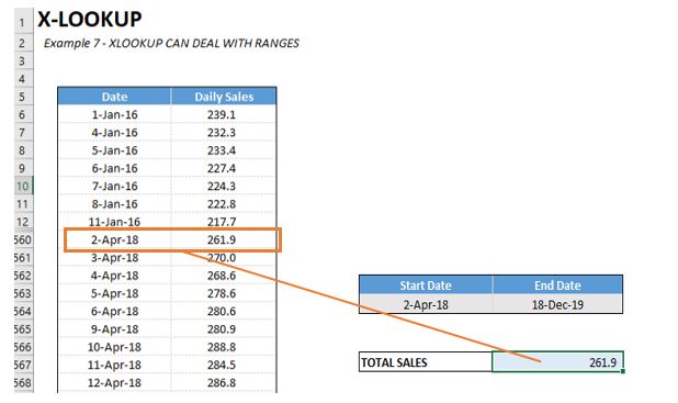
The Output 261.9 is the sales for 2^nd April 2018 (ie; start date).

To get the result of the full range we will have to press F2 and Edit the formula.

Press F2 and add a Colon (:) as we type normally for a range in excel.

Then extend the formula for the END DATE. (SEE BELOW HIGHLIGHTED IN BLUE)

XLOOKUP(F7,$B$6:$B$1088,$C$6:$C$1088):XLOOKUP(G7,$B$6:$B$1088,$C$6:$C$1088)

Lookup_value is the END Date. Link it to “Cell G7”

Lookup_array is the Date Range in the second table (B6:B1088)

Return_array is the Daily Sales (C6:C1088)

Fix the ranges B6:B1088 and C6:C1088 using F4 function key.

NOW Since we want to get the total sales during the select period type SUM to the start till end of the XLOOKUP formula [Like = SUM(XLOOKUP():XLOOKUP()] – SEE BELOW

=SUM(XLOOKUP(F7,$B$6:$B$1088,$C$6:$C$1088):XLOOKUP(G7,$B$6:$B$1088,$C$6:$C$1088))

You get the following output for the selected range.

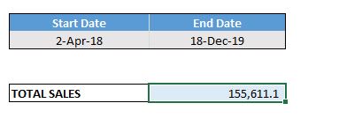
If you want to check it. You can select the range and check the total at the bottom of the window (as shown below).
 

Example 8

SUPPORTS WILD CARDS FOR PARTIAL MATCHES

Here is the data set showing employee ID, Name and their Annual salary.

 

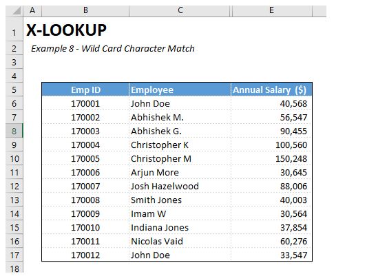
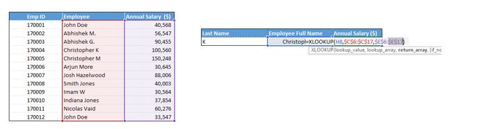
Suppose we just remember the last name of the employee and we want to pull the full name and Annual salary from the database.

Is it possible?

 

Yes, now it is possible with XLOOKUP Function

We can use Wild Card Feature for Partial Mismatches in XLOOKUP Function.

Lets learn how to use it.

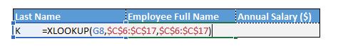
TYPE XLOOKUP(

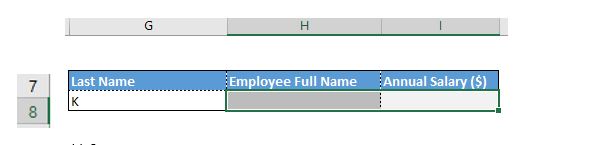
Lookup_value is the Last Name. Link it to “Cell G7”

Lookup_array is the Range (C6:C17)

Return_array is again the same Range (C6:C17)

Fix the ranges C6:C17 (both instance) using F4 function key.

Leave other function arguments blank, Close the bracket and then press OK.

You get an error.

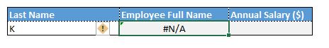
This is because now XLOOKUP is doing an exact match.

To use Wild Card/ Partial mismatch, type an asterisk (*) within inverted Commas like this “*” followed by & before lookup value.

We also need to use the fifth argument here which is the “Match Mode” where we will use 2 which used for Wild Card character match.

Now edit the front and back portion of the formula like this =XLOOKUP(“*”&G8,$C$6:$C$17,$C$6:$C$17,,2)

Click Enter.

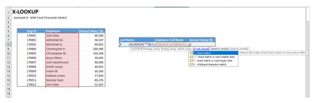
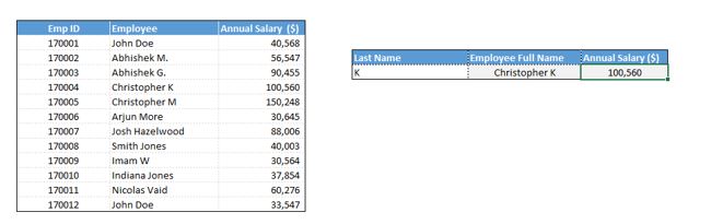
You get the following Output.

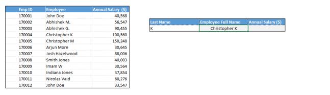
Now you can link the next XLOOKUP function to the Full Employee Name or again use the Wild Card match to pull the Annual Salary.
 

Here I am using the Full Employee Name to pull the salary (as we discussed in our previous examples).

Here is our output.

This is how we can use wild card/partial match option to pull data from large databases. This was not possible using VLOOKUP or index/match functions earlier.

We have covered all the functionalities of XLOOKUP function. Let us know if you have any questions/ comments by posting in the comments section.

Keep learning. Have fun.

Our Data analytics in Excel online course , will provide more hands on training to you to get expertise in Excel functionalities.

We also provide a comprehensive financial modeling and business valuation skills online course, to get you trained as a Financial Analyst.

This 5 mins read will inform you more about Microsoft Excel as a tool for Data Analytics.

Hope you enjoyed learning. Have fun.