Excel Data Analysis 101: 9 Essential Data Manipulation Techniques

Data analysis is a challenging task, especially if you don’t have the data manipulation skills. In this article, we will discuss some of the most common data manipulation techniques that can be used in Excel for data analysis.

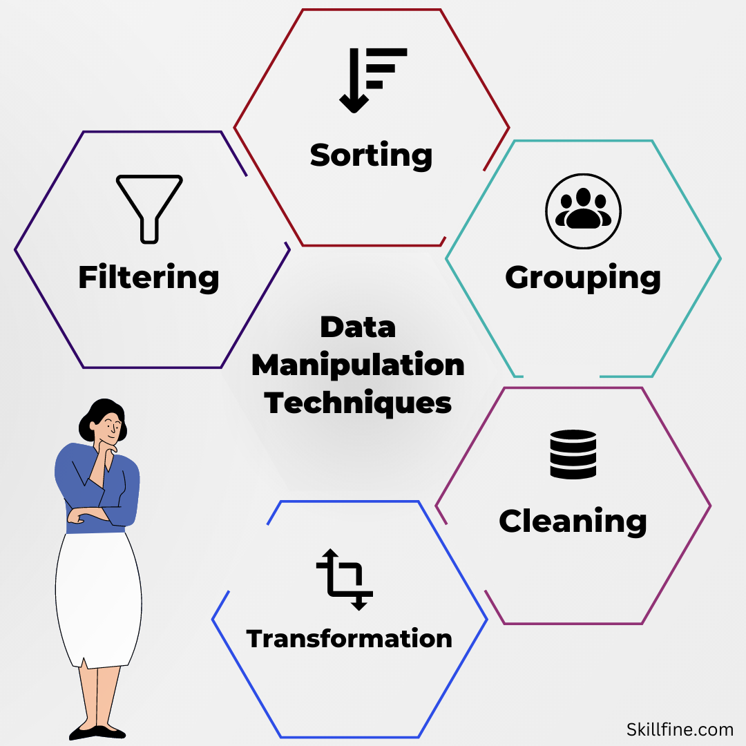
The power of these techniques will be demonstrated by using some real-life examples. The 9 common data manipulations techniques discussed are:

1) Filtering

2) Sorting

3) Grouping

4) Pivoting

5) Transposing

6) Changing Data Types

7) Adding Columns and Rows

8) Naming Columns or Rows

9) Inserting Columns or Rows.

Each of these techniques will provide you with a better understanding of your data and how it works – from getting your head around different types of visualization to exploring outliers. These simple tricks will not only improve your efficiency, but also make it easier for people who don’t know Excel as well to understand what you’re doing.

Filtering

Filtering is a process of sorting data by a certain criteria. It’s an effective way to identify subsets of data from the larger dataset.

In the following example, we have a dataset with monthly sales data from 2012-2015. Filtering is useful if you want to see the total sales for the year only, or if you want to know how many months had positive growth.

First, identify which column contains the filter criteria that will be used to filter your data. In this case, I have created a new column called “Sales Growth.” Next, highlight your “Sales Growth” column and select “Filter” from the Data menu on the toolbar. This will open a dialogue box where you can input your filtering criteria. In this example, I am using “>0%” as my filter criterion to calculate total sales for years with positive revenue growth > 0%.

Sorting

Sorting is another technique of data analysis and is used to rearrange the order of your data. It’s an easy way of exploring and understanding your data.

For example, let’s say you had a list of 5 different numbers:

1, 10, 2, 3, 4

If we wanted to sort this list in ascending order (from lowest to highest), we would click on the column heading for this list and then select “Sort Ascending”. This will arrange the list like this:

1, 2, 3, 4, 10.

By sorting the numbers in ascending order we can see that they are increasing in size. If we wanted to change the sort order to descending (highest to lowest) we would click on Column A and select “Sort Descending” like so:

4, 3, 2, 10, 1.

Again by sorting in descending order from highest number to lowest number we can see that they’re decreasing in size.

Grouping

Grouping is an excellent way to analyze your data. Grouping is when you organize data into smaller sets. You can use this technique to make it easier to analyze the relationships in your data like quantifying averages, totals, and percentages.

Grouping makes it easy for you to identify patterns in your data. For example, if you wanted to know how many people are in each age group (20-25, 26-30 etc.), then you can group that information by age group and then count the number of people in each one.

The best thing about grouping is that it helps you quickly identify relationships in your data set because it shows you which items are grouped together. This means that if there’s a trend between two different groups of data, then grouping will be able to show you this connection.

Pivoting

Pivoting data involves taking a table and turning it on its side to show a different perspective.

For example, let’s say you have a list of monthly income brackets and want to see the monthly income distribution for each bracket. You can do this by pivoting your table from column to column.

In our example, we would start with one column containing all of the monthly income brackets. In the next column, we would add a pivot table that contains the percentages for each income bracket.

Pivoting is very helpful in filtering out irrelevant data so you can focus on the important information. If you have a huge dataset, extracting relevant information can be time-consuming without using pivots.

If you’re looking for a way to simplify data analysis in Excel, pivoting is an effective tool!

Transposing

Data can be transposed by using the TRANSPOSE function in Excel. It is a very efficient way to take any data, for example:

5 10 15 20 25 30 35 40 45

and turn it into this:

1 5 10 15 20 25 30 35 40 45

This is helpful when you want to switch rows and columns or swap columns or rows with each other.

Changing Data Types

One thing that might be useful to know is how changing data types can affect your data analysis.

Two different types of data are text and number. Text data is any kind of information that isn’t numerical. For example, a person’s name or the title of a book. Numberic data will always be numerically based and may only have numbers in them, such as 3.1, 4.9, and so on.

If you want to change the type of your data from one type to another, you will need to use the function Data→Data Type→Text or Number.

Changing Data Types

Once you select this command, the “Select Data Type” window will appear. There are three general categories of data: Text Data

only; Numeric Data only; and Mixed Data (text and numeric).

You can further refine your selection by selecting one or more options from each of these categories: Text; Numeric; Date & Time; Logical; and Object Linking & Embedding

Adding Columns and Rows

Adding columns or rows to your data is a great way to make your work more efficient. For instance, if you were working with a table of data on different subjects and wanted to look at their answers in relation to each other, it would be more convenient for you (and the people you’re sharing the data with) if you had both answers in one column.

Naming Columns and Rows

To name columns and rows in Excel, first select the cells that need naming. Then go to Data > Data Tools > Name Columns and Rows and type the name of the first cell into the first dialogue box. Continue typing or clicking until all of your cells are named.

Naming Columns or Rows

Every column and row in a spreadsheet has a default name, but these names can be changed. This is helpful when you’re summarizing data and want to apply the same column or row title consistently.

To rename a column, right-click on any cell in that column and select “column name.” Type in the new name and press enter. To rename a row, right-click on any cell in that row and select “Row Labels.” Type in the new name and press enter.

Inserting Columns or Rows

One of the simplest data manipulation techniques in Excel is inserting columns or rows.

This technique lets you analyze your data with more clarity and precision by adding more columns or rows to your spreadsheet. It can be used to show different aspects of your data, such as different years, regions, products etc.

Two examples where this technique can be used are:

1) You want to compare different years for a specific region. 2) You want to look at how a product performs across different regions.

Conclusion

Data manipulation can be a time-consuming and complicated task. But the right technique can help you save a lot of time and avoid making mistakes. The 9 basic techniques in this article can help you navigate data manipulation in Excel.

Excel Data Analysis 101: 9 Essential Data Manipulation Techniques