The Indirect function returns the reference specified by a text string. It is used to indirectly reference cells, ranges, other sheets within the same workbook or a different workbook. Instead of hard coding a cell or range, Indirect function helps to create a dynamic cell or range reference. Hence one does not need to change the formula itself and instead can change a reference within a formula thereby making it a super dynamic function. When a new row or column is inserted or deleted in the worksheet these indirect references will not change. The Indirect function does not evaluate any conditions or logical tests. It also does not perform any calculations. This function simply helps to lock up the specified cell in a formula.

SYNTAX

The Indirect function has two arguments out of which the first argument is required and second one is optional.

= INDIRECT (ref_text, [a1])

Where,

ref_text (required): is a reference to a cell that contains and A1 or R1C1-style reference, a name defined as a reference, or a reference to a cell as a text string.

A1 (optional): is a logical value that specifies the type of reference in Ref_text argument:

• R1C1-style = if FALSE, ref_text is treated as a R1C1 reference
• A1-style = if TRUE or omitted, ref_text is treated as an A1-style reference. This is the default option.

Note: We mostly use the most familiar A1-style of referencing, though R1C1 may be useful in certain situations. Usually we cannot use both the styles in a single worksheet at the same time. To switch between the two reference types, we have to go to File> Options> Formulas> and tick the R1C1 check box.

BASIC EXAMPLE OF HOW INDIRECT FUNCTION CONVERTS A TEXT STRING INTO A CELL REFERENCE

Let’ take a very simple example of this. We write a number say 5 in cell A1 of an excel sheet, and then write down the cell reference A1 in cell C1. In cell D3 we want the value in cell A1. Here we can use Indirect function as below.

=INDIRECT(C1)

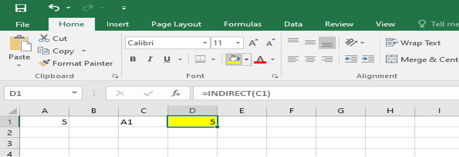
We can note here that the Indirect function here refers to the value in cell C1, which is A1 and the function routes to cell A1 where it picks up the value to return i.e., 5. Hence, Indirect function converts a text string into a cell reference.

UNDERSTANDING A1 AND R1C1- STYLE OF REFERENCING

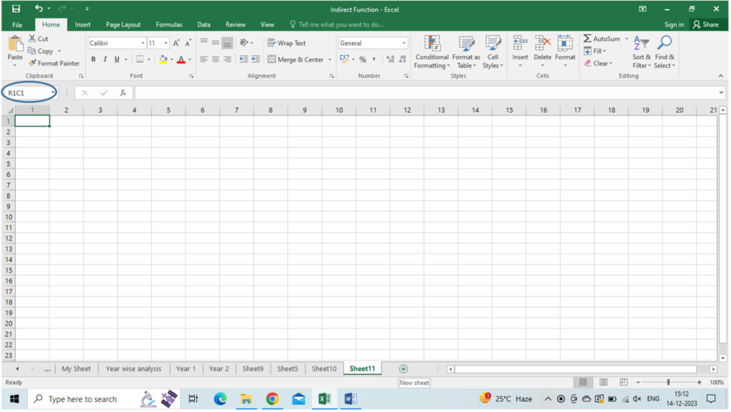
As discussed above if we switch to R1C1 style of referencing through File> Options> Formulas> R1C1 check box style, then we get excel sheet as follows. We can see that instead of the regular name of cell as A1 in the name box we get the name as R1C1 in the name box.

Let’s see through an example how to use A1 and R1C1 references in excel in A1 default mode.

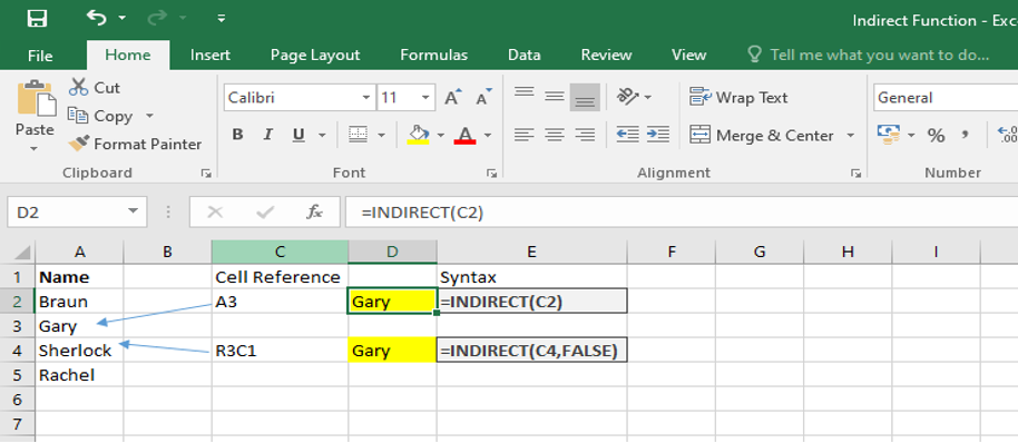
Example: We want to get the name in row 3 of column A.

Syntax in A1 style

=INDIRECT(C2)

A1 style of referencing is the default type in Excel that refers to the column followed by row number. For example, here it refers to the cell at the intersection of column C and row 3. The Indirect function here converts the text string in cell C2 as a cell reference, heads to A3 and fetches the result Gary.

Syntax in R1C1 style

=INDIRECT (C4, FALSE)

R1C1 style of referencing is just the opposite of A1 style were the row number is followed by the column name. For example, here R3C1 refers to row 3 and column 1 in the sheet. FALSE in the function refers the second argument which says that the function should be treated like a R1C1 style referencing. Hence the function fetches the value from Row 3 and column 1 i.e., Gary.

INDIRECT REFERNCES CREATED FROM CELL VALUES AND TEXT

We can use Indirect function by combining a text string and a cell reference within our Indirect function by using concatenation operator (&).

Example: We have a number in cell B2 and we have the row number of cell B2 i.e., 2 in cell C2. We want to create an Indirect function combining both text string and cell reference.

The Indirect function combines the two elements in the ref_text argument as text B in double quotation and the value in cell C2. The combined text string and cell reference gives reference to cell B2 and returns the value of cell B2 i.e., 5 in cell D2.

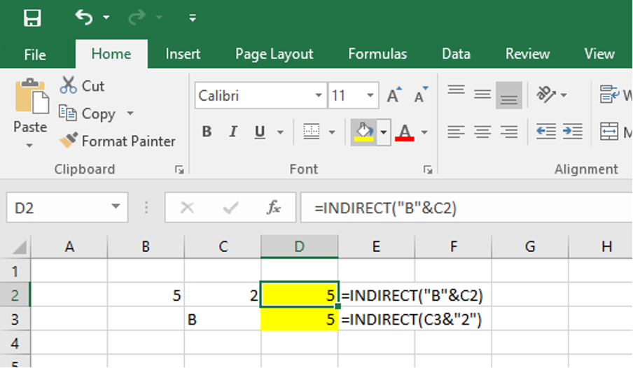
In the above example if we use cell reference in cell C3 and text string as “2” using concatenate function, we will get the same result in cell D3.

INDIRECT FUNCTION WITH NAMED RANGES

Apart from using Indirect function to make references from cell and text values, we can also use it to refer to named ranges.

Example: Suppose we have a few students studying in a university and each student secures certain marks in each of the four subjects. The teacher wants to find the students average marks secured and total marks in all the subjects.

We can simply apply sum and average function to get the marks of each student. However, in order to make the calculation more dynamic we will use the Indirect function combined with drop down list.

The table of students marks against the subjects are given below:

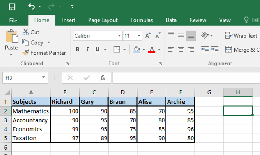
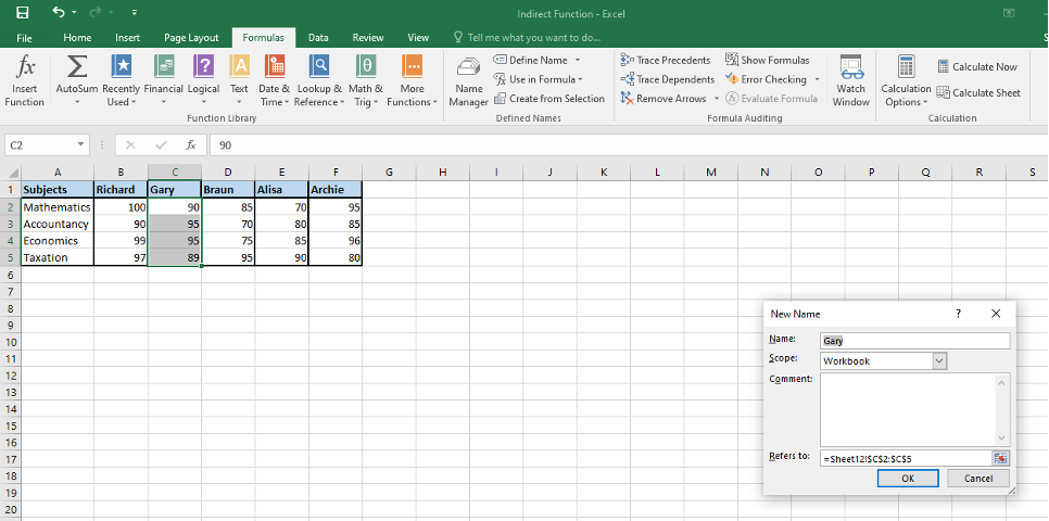
Next we have to rename the cells. Each cell in excel has its unique address, for example in the above example the cursor is at cell H2 and the address is displayed in the name box just above the cell A1 in the left most corner. We can however change the name of the cell or a range of cells by simply selecting the cell or cells we want to rename, go to the name box, type the new name and press enter. We can also change the name of cell or range of cells by going to formula tab in excel > Defined names> Define name> OK.

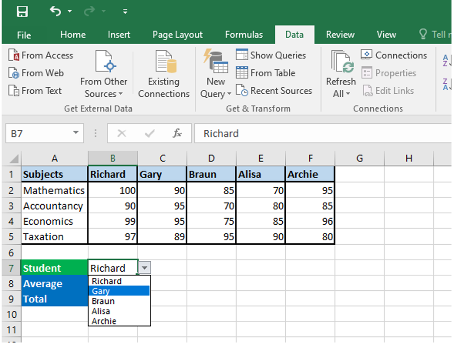
Once we have renamed all the cell range with the names of the students, we can create a drop down list of students in cell B7. To create drop down list go to data tab> data tools> data validation> settings tab> under allow option select list> select the source of names from cell B1:F1.

Once the dropdown is created we can calculate the average and total marks of each student in a dynamic way using the indirect function as below. We can use indirect function to refer to the cell B7 containing the names of the students in a drop down list as below.

We can embed the indirect function with cell reference to B7 with any other excel functions to find the sum, average, minimum, maximum or any other calculations of the named ranges as below:

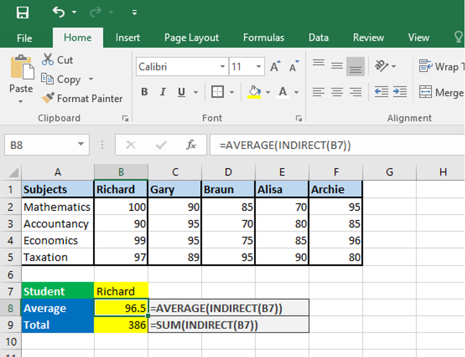
This data set is super dynamic. We can find the average and sum total marks of any student by just changing the name from the drop down list, and here we have the calculations within a fraction of second.

INDIRECT FUNCTION TO REFER TO ANOTHER WORKSHEET

We can also use the Indirect function to refer to the cells on another worksheet, instead of referring to cells on the same worksheet as discussed in the above examples. We will discuss this with the help of an example which can be used in the financial modelling purpose.

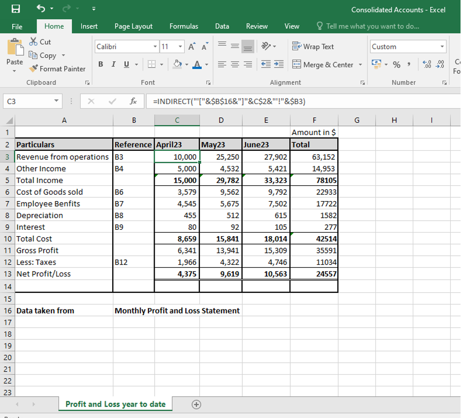
Example: A company prepares monthly Profit and Loss statement and then consolidates the profit year to date every month to check what is its net profit or loss till date. To explain here in short, we will take Profit and loss statement of only first quarter of the year, and try to calculate the net profit or loss for the quarter 1.

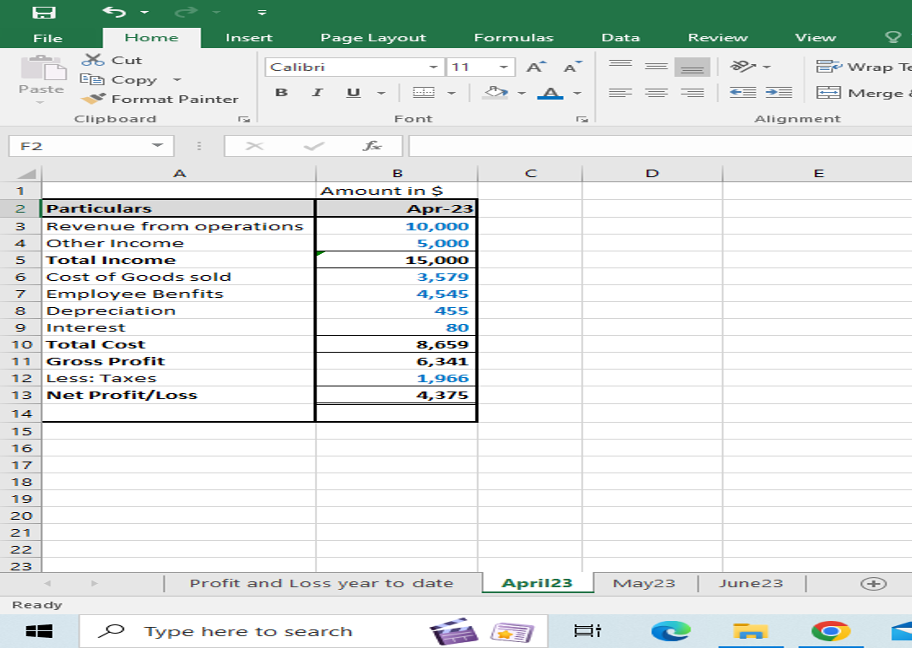
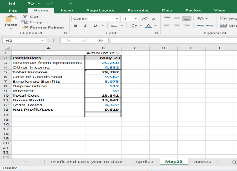
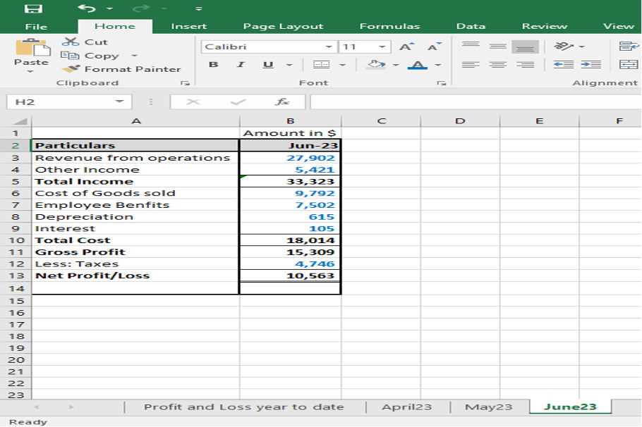
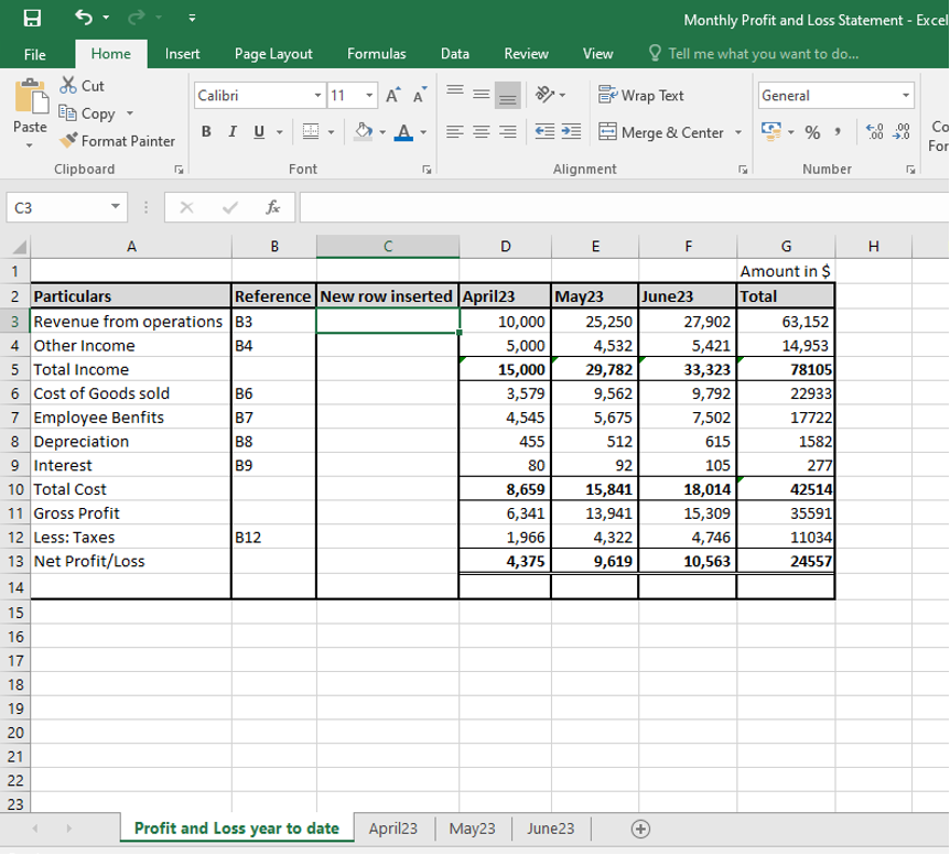
In the below example we have profit and loss statement of three months- April23, May23 and June23 in three different worksheets, and we want to calculate the total profit and loss for the quarter by pulling the data for all the three sheets in the worksheet named Profit and Loss year to date. The three month wise excel worksheets appears as below. The figures in blue are hardcoded figures and those in black are formula driven.

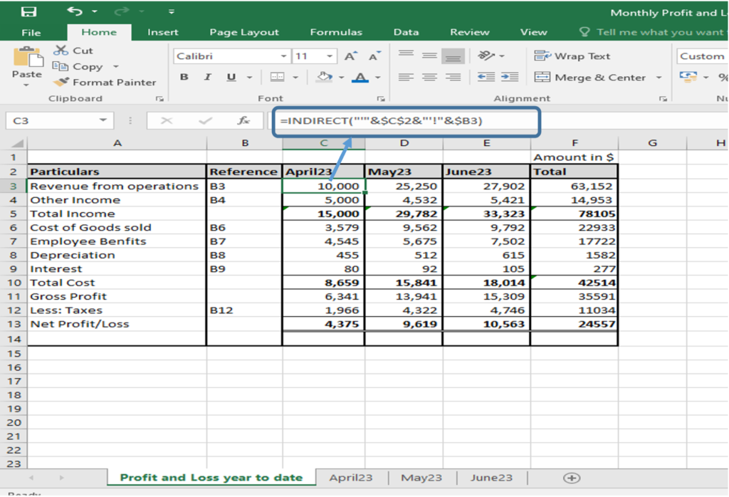
We want the total profit and loss in the sheet named Profit and Loss year to date. For this will we use Indirect function.

We will break the formula in the screenshot and understand this in detail.

We usually reference another worksheet in excel is by writing the worksheet’s name followed by the exclamation mark and a cell / range reference, like SheetName!Range. We should enclose the sheet name in single quotes to prevent an error since the sheet name often contains a space(s). For example, when we want to extract the revenue from operations figure from the April23 sheet we will write: ‘April23’!B3. By writing this the Indirect function shall search for April23 worksheet and cell B3 in that worksheet to get value in the main sheet.

To make this more dynamic and to apply this formula to pull figures for other two months too, we shall enter the sheet names as the header in cell C2, D2 and E2, the cell address from where the data is to be pulled from month-wise sheets in the reference column, concatenate them in a text string and put that string in the Indirect function. Note that here we have maintained the Particulars of all the three months in the same format and same cell range so that we can dynamically pull the data in the main sheet and using the same reference no. Important point to remember here is that in a text string, we have to enclose all the elements in double quotes except the cell address or a number, and link all the elements in the text string using the concatenation operator (&).

Having explained the above example, we get the Indirect function as below:

INDIRECT (“‘” & Sheet’s name & “‘!” & Cell to pull data from)

In the above example, to pull the revenue from operations figure in the main sheet, we will enter the following formula in the cell C3:

=INDIRECT(“‘”&$C$2&”‘!”&$B3)

Where,

• The sheet name in linked to cell C2. We have locked the reference to the sheets name using the absolute referencing like $C$2 since we will be also pulling down the formula to other particulars like Other income, cost of goods sold etc.
• We have enclosed the single quotes and exclamation mark in double quotation.
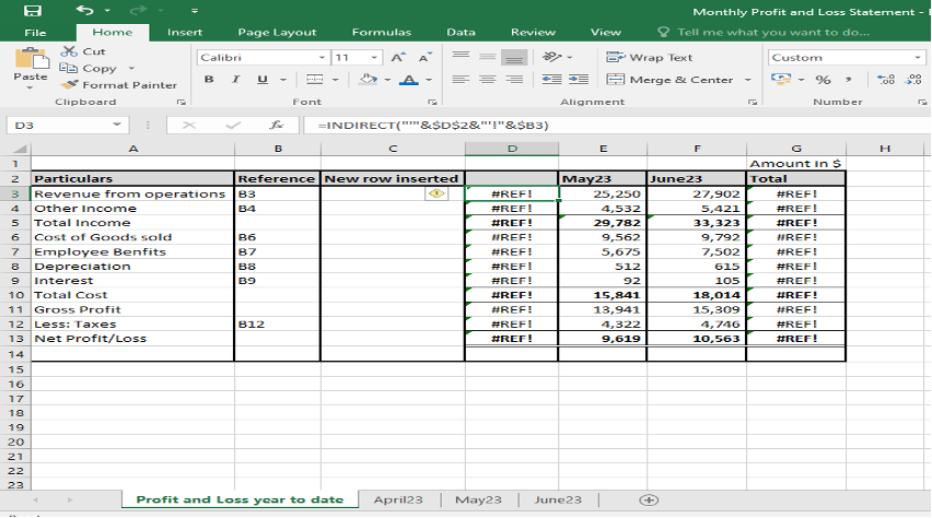
• The cell reference to pull data is linked to cell B3 with text written as B3. Note that even if we insert a new column next to the reference column we will get the same result as before. Hence, Indirect function helps to lock a cell reference, and remains unaffected due to addition or deletion of any row or column.

Points to note:

1. If either the Sheet name (for example April23 in cell D3 or the reference (for example cell B3 in the Profit and loss year to date sheet is empty, then the Indirect function shall return an error. To prevent this, we can wrap the indirect function in the IF function as below. For example, in the above example April 23 is missing from the cell D3, we get the following:

 To prevent this error, we will write the following syntax:

=IF (OR (D$2=””, $B3=””),””, INDIRECT(“‘”&$D$2&”‘!”&$B3))

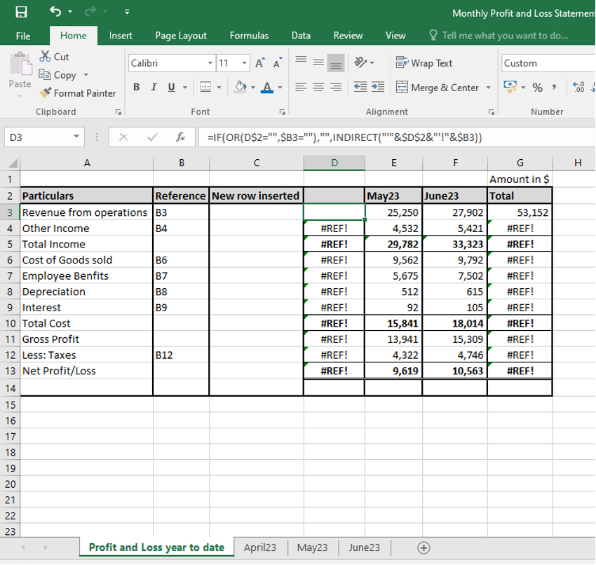
We can pull this formula to the rest of the cells to remove error.

• If the referred sheet is closed the Indirect function shall show a #Ref error. To avoid this, we can use the IFERROR function which will show a blank i.e., an empty string wherever an error occurs.

Syntax: =IFERROR(INDIRECT(“‘”&$D$2&”‘!”&$B3),””)

INDIRECT FUNCTION TO REFER TO ANOTHER WORKBOOK

This is similar to Indirect function referring to another worksheet in excel. The only addition here is that we have to enter the workbook’s name in addition to the worksheet’s name and the cell address.

When the book name contains a space we have to use apostrophes in the place of the space. The string will look like: ‘[Book_name.xlsx]Sheet_name’!Range

For example, the Main sheet i.e., the Profit and Loss year to date sheet referred to in the example above is in another workbook named Consolidated Accounts as below:

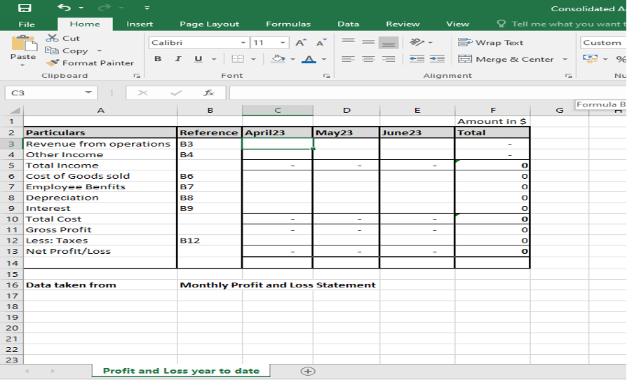
We want to pull the month wise data in the workbook named Consolidated Accounts from the workbook named Monthly Profit and Loss Statement. For this we may write the workbook name from where the data is to be pulled in a separate cell B16. The sheet name is mentioned in cells C3, D3 and E3 and the cell address in the column named Reference. Given all the inputs we can pull the revenue from operations for the month of April23 in cell C3 as below:

=INDIRECT(“‘[“&$B$16&”]”&C$2&”‘!”&$B3)

We should lock the cell containing the workbook name and worksheet name using absolute cell referencing since we do not want the cells to change while copying the formula to other cells.

Hence, in general the syntax for using Indirect function to reference to other Excel workbook is as follows:

=INDIRECT (“‘[” & Book name & “]” & Sheet name & “‘!” & Cell address)

Points to note: If the workbook being referenced to is closed the Indirect function shows up a #Ref error. To avoid this error, IFERROR function can be used with the Indirect function.

=IFERROR(INDIRECT(“‘[“&$B$16&”]”&C$2&”‘!”&$B3),””)

INDIRECT FUNCTION USED WITH OTHER EXCEL FUNCTIONS

Indirect function as demonstrated above is a very dynamic function and can be used along with other functions apart from sum and average functions like- row, column, Vlookup, address functions to name a few.

USING INDIRECT FUNCTION WITH ROW FUNCTION

ROW function is used to return an array of values in excel. To return the average of the 4 smallest numbers in the range A1:A15, we can use the following array formula. The formula after being entered requires pressing Ctrl+ Shift+ Enter.

=AVERAGE (SMALL (A1:A15, ROW (1:4)))

Similarly, the sum of smallest 4 figures in the range can be found as:

=SUM (SMALL(A1:A15,ROW(1:4)))

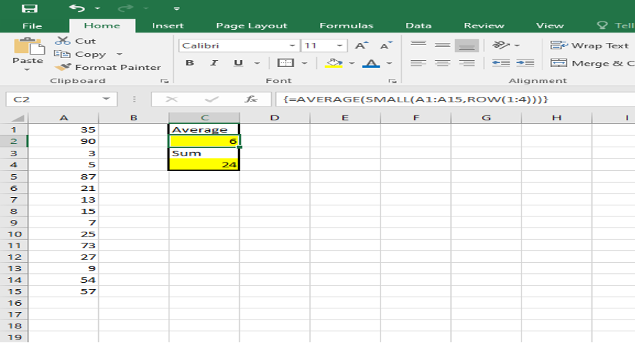
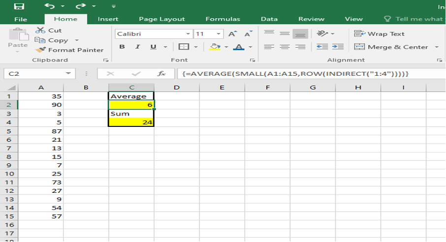
However, if we insert any row in between the range selected between the rows 1 and 4, the range in the ROW function gets automatically changed to ROW(1:5) and the formula returns an average or sum of 5 smallest numbers instead of 4. Hence, to prevent this from happening, we can use the Indirect function and no matter how many rows are inserted or deleted the array function will always give us the correct result.

=AVERAGE (SMALL (A1:A15, ROW (INDIRECT (“1:4”))))

=SUM (SMALL (A1:A15, ROW (INDIRECT (“1:4”))))

Similar, to this we can use a combination of large function along with row and Indirect function.

USING INDIRECT FUNCTION WITH VLOOKUP FUNCTION

Let’s understand with the help of an example.

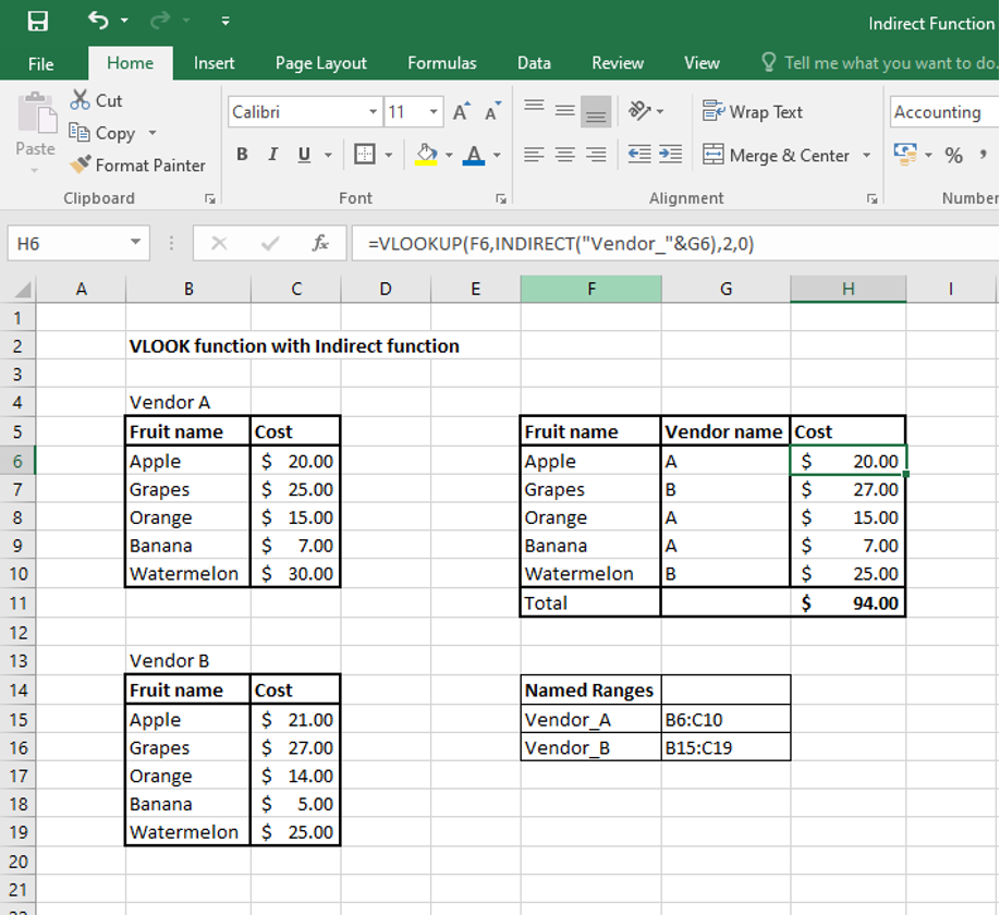
We have list of two vendors supplying some fruits and both the vendors are supplying the fruits at different prices. We want to calculate the total cost of purchasing the fruits from two of the vendors in a single table. We will pull the cost of fruit against each vendor using VLOOKUP function combined with the Indirect function as below.

=VLOOKUP (F6, INDIRECT(“Vendor_”&G6),2,0)

CONCLUSION

We have seen that the Indirect function is a very dynamic function and one can easily incorporate the Indirect function along with other excel functions to make their Excel dashboards and Financial Modeling templates more easily to use and automated.

Check out this blog on our LinkedIn page as well: