Imagine playing with a set of building blocks. You can either stack them on top of each other to make a tower or lay them side by side to build a wall. When working in Excel, your data often resembles those blocks—sometimes you need to combine this data vertically, other times horizontally. Luckily, Excel’s VSTACK and HSTACK functions make this task simple and efficient.
VSTACK and HSTACK are relatively new functions, designed to help you consolidate data in a few keystrokes. They can significantly cut down on manual tasks like copying, pasting, and rearranging data. In this article, we’ll explore how to use these functions, provide complex real-world examples, and show you how to integrate them with other Excel formulas for maximum productivity.
Whether you’re a beginner or an advanced Excel user, this guide will help you master VSTACK and HSTACK, boosting your data manipulation skills. Additionally, you will also learn how to write good ChatGPT prompt to help you use VSTACK() and HSTACK() and their alternative functions with no hassle! Here’s our examples sheet for you to follow along: VSTACK and HSTACK examples.xlsx.
1. Understanding the Basics of VSTACK and HSTACK
VSTACK: Think Vertical Like a Skyscraper
The VSTACK function allows you to stack data on top of each other, combining multiple arrays or ranges of data into a single vertical column. If you think of your data like a stack of books, VSTACK would be the tool that neatly piles one dataset on top of another, saving space and giving you a clean, consolidated view.
- Real-Life Scenario: Picture this – You’re a sales manager tracking quarterly sales data for your team. In January, you’ve got numbers from your East and West teams, and in February, you’ve got the same data. However, the CEO wants a full list that shows both teams’ performances in one vertical column so they can analyze total sales. Instead of copying and pasting data manually, VSTACK does the heavy lifting for you. It takes the two columns and stacks them one on top of the other like a single report card for all your teams!
- Syntax of VSTACK:
=VSTACK(array1, [array2], …)
- Example: Imagine you have sales data for Quarter 1 in column A and Quarter 2 in Column F, and you want to merge them into one column. VSTACK combines the two arrays of data into a single vertical stack.
=VSTACK(A1:A5, F1:F5)
HSTACK: Horizontal Like a Bookshelf
Now, let’s talk about HSTACK. Just like its counterpart, HSTACK also combines data, but instead of going vertically, it arranges your data side by side. Think of it like a bookshelf where you neatly place books next to one another so you can easily see all the titles.
- Real-Life Scenario: Imagine you’ve got a list of your company’s products in one column and their corresponding prices in another. You want to create a summary where each product is listed next to its price for easy comparison. HSTACK allows you to line up the data horizontally, creating a single row for each product-price pair.
- Syntax of HSTACK:
=HSTACK(array1, [array2], …)
- Example: If you have patient names in column A and their guardian’s name in say, column B, you can combine them into a single row like this:
=HSTACK(A1:A5, B1:B5)
Both functions are particularly useful when consolidating datasets from different sources or when you need to prepare data for reporting purposes.
**
2. Practical Examples of VSTACK in Action
To get a real sense of how powerful VSTACK can be, let’s explore five unique, real-world examples. Each demonstrates a specific way these functions can save time and simplify data management.
Example 1: Creating a Dynamic Stacked List
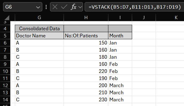
You have a dataset with information on doctors, the number of patients they treated, and the corresponding month and year in which they got treated. The data is structured in three tables, each representing a specific month in 2023 (January, February, and March), with doctor names and patient counts repeated across these months.
Situation:
You can use VSTACK to vertically stack these groups into a single column for 3 fields (Doctor Name, No. of Patients, Month)

Hospital Info 2023
Formula:
=VSTACK(B5:D7,B11:D13,B17:D19)
Result:
Result of using VSTACK()function
What Happens:
VSTACK(B5:D7,B11:D13,B17:D19)
- VSTACK takes the products from the first 3 columns of Table 1 (B5:D7), Table 2 (B11:D13) and Table 3 (B17:D19) and stacks them into a single column.
Why is this Useful?
- Efficiency: This formula saves you from having to manually go through multiple lists, and combining them.
- Automation: If the lists are updated (new data are added to any table), the formula will automatically update the combined llist—making it dynamic and easy to manage over time.
**
Example 2: Combine Data From Different Sheets with VSTACK()
Situation:
Let’s say we have the same data as in example 1, but this time we wish to consolidate dynamic data from another sheet as well. Let’s look at how we can achieve that.
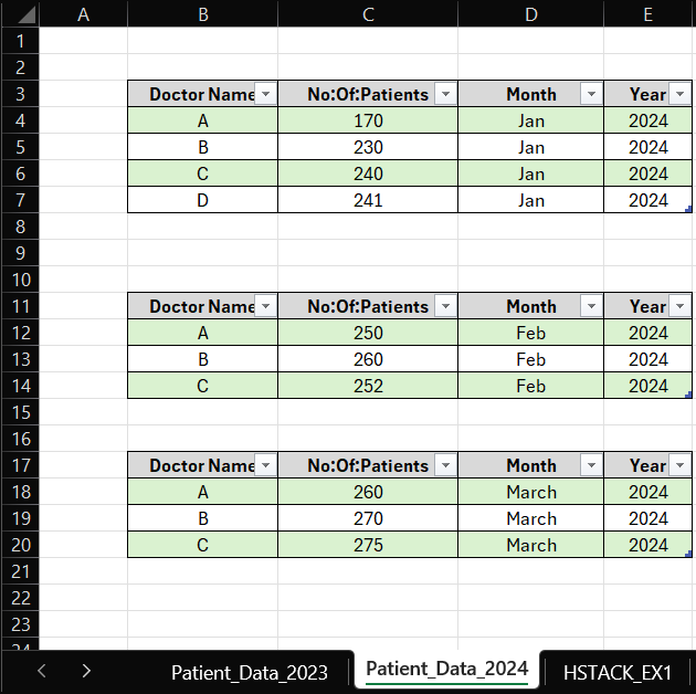
Patient Data 2024
Formula:
=VSTACK(Table1,Table2,Table3,Table16,Table28,Table310)
Where
Table1 – Patient_Data_2023!B5:E7
Table2 – Patient_Data_2023!B11:E13
Table3 – Patient_Data_2023!B17:E19
Table16 – Patient_Data_2024!B4:E7
Table28 – Patient_Data_2024!B12:E14
Table310 – Patient_Data_2024!B18:E20
Note: This formula is being pasted in a cell of the Patient_Data_2024 worksheet.
To create dynamic tables, select the desired data range with header included and navigate to Insert > Table. Once the dialog box opens, verify if the data range is correct and check the ‘My data has headers’ checkbox. Your table will now be be created with a default name. This is how the tables in the above formula were created.
Result:
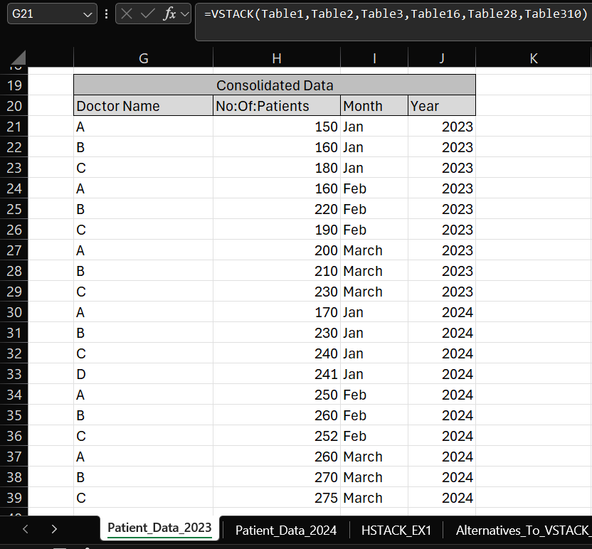
Consolidated from two sheets with VSTACK()
Why is this Useful?
- Efficiency: Instead of manually copying and pasting data from multiple worksheets, VSTACK combines them into one list with a single formula.
- Dynamic Capacity: If you update or add new data in any of the sections (like adding April data), the formula will automatically include the new data, keeping the list dynamic and easy to manage.
**
Example 3: With VSTACK() and SORT()
Situation:
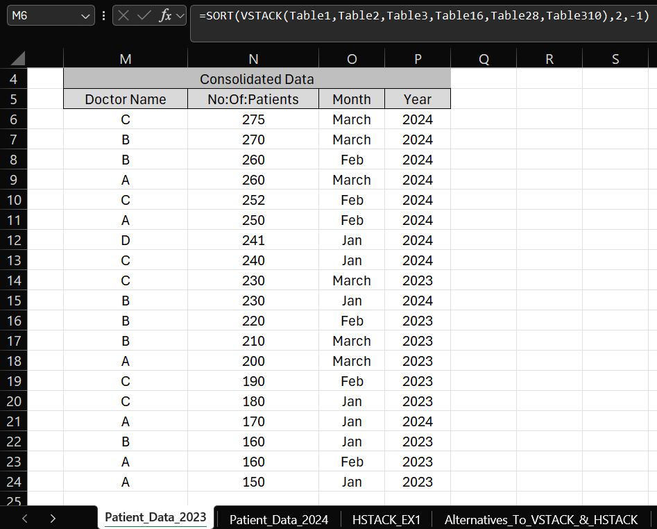
For the same data, we wish to consolidate dynamic data from different sections of the same worksheet and sort it by the “No:of:patients” column in a descending order.
Formula:
=SORT(VSTACK(Table1,Table2,Table3,Table16,Table28,Table310),2,-1)
Result:
VSTACK() with SORT() on Patient Data
Limitation:
This example is particulary useful when you’d like to sort the resultant data. When you use functions like VSTACK() or HSTACK(), Excel creates a dynamic array that spills the results into adjacent cells. This means that the output of the function occupies multiple cells as one single entity. You cannot edit individual cells of this output directly. When you try to sort or otherwise manipulate part of a dynamic array directly using the SORT or FILTER options on the UI for specific columns, Excel gives you the error “you can’t change part of an array” because it requires you to work with the entire array. The most efficient way to handle this is to use enclose the entire resultant array data range in a SORT(), FILTER() or other functions of choice as a formula.
**
3. Practical Examples of HSTACK in Action
Example 1: Merging Project Data (HSTACK)
Situation:
You have project data, such as project names, start dates, and end dates in one table and info about the people involved in the project. You want to merge this data into a single row.
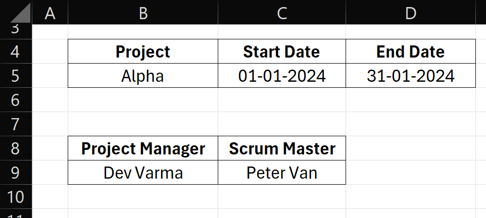
Project Data
Formula:
=HSTACK(B5:D5,B9:C9)
Result:
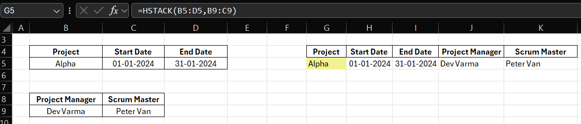
Result of using HSTACK on Project Data
Please note that in some cases, you may have to format some columns to a specific datatype in your resultant data array. For example, the date columns may have to be changed to a SHORT DATE or LONG DATE format as per your requirement after stacking. By default, the HSTACK() applies a General format for all the data values.
Why is this Useful?
- Clear Presentation: Merging project-related data into a single row gives a clear, organized view of each project and its timeline. It allows you to view all key information at a glance.
- Data Consolidation: It consolidates scattered data (in separate columns) into one continuous row, making the data easier to copy, export, or use in reports.
- Quick Analysis: This approach helps in quickly analyzing timelines for multiple projects, without flipping through multiple columns or sheets. For example, if you had the two tables shown above in two different sheets, the HSTACK() function would make it so much more easier to consolidate everything and perform advanced analytical tasks.
**
Example 2: Using HSTACK() to combine data from multiple sheets
Situation:
Let’s use an example of combining data from multiple sheets related to Employee Information and Project Assignments for a tech company. This illustrates how to use the HSTACK() function to combine data across different sheets – We want to create a summary that combines employee details with their current project assignments, even when the Employee IDs are in different orders.
Sheet 1: Employee Information

Sheet 2: Project Assignments

Although HSTACK() combines arrays horizontally, it does not inherently handle different ID orders. Instead, you would typically combine data after ensuring that the IDs match. We can achieve the desired summary by sorting both sheets by Employee ID first and then using the HSTACK() function to combine the data. Sorting the data ensures that the Employee IDs are aligned correctly, making it straightforward to combine the information.
Formula:
=HSTACK(SORT(Table6, 1, TRUE), SORT(Table10[[Project Name]:[Status]], 1, TRUE))
Where
Table6 = Employee_Data!B6:E10
Table10 = Project_Data!B6:E9
This formula is pasted in a cell in a third sheet called Project_Summary.xlsx
Result:
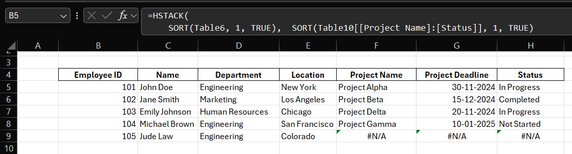
Summary Sheet Data using HSTACK() and SORT()
As you can see, the consolidated data is now available in the summary sheet and whenever corresponding data is not available for an Employee ID in either of the sheets, the associated column values are filled with “#N/A” by default.
Why this is useful:
- Comprehensive Overview: You get a holistic view of employee information and their project assignments in one table with exact matches of the identification column values.
- Dynamic Updates: If any data in the employee or project sheets changes, the summary updates automatically.
- Simplified Reporting: Makes it easier to generate reports for team meetings or project updates.
This example shows how you can use HSTACK() to effectively combine data from different sheets in Excel, providing a clear and organized summary.
Now, one may ask – this can be achieved by VLOOKUP() or INDEX() and MATCH() as well. So why use HSTACK()?
Let’s say, if we were to achieve the same result as above using VLOOKUP, we would have to use a separate VLOOKUP formula for each column in our summary sheet as shown below. If there were a 100 columns, this would be a tedious job.
=VLOOKUP(B5, Table6, 2, FALSE) -> For Name Column
=VLOOKUP(B5, Table6, 3, FALSE) -> For Department Column
=VLOOKUP(B5, Table6, 4, FALSE) -> For Location Column
=VLOOKUP(B5, Table6, 5, FALSE) -> For Project Name Column
=VLOOKUP(B5, Table6, 6, FALSE) -> For Project Deadline Column
=VLOOKUP(B5, Table6, 7, FALSE) -> For Status Column
When to Use HSTACK():
- If your goal is to present multiple datasets side by side and you can ensure the data will be in order, HSTACK() can be very effective for simplicity and clarity.
- It works best in scenarios where you want to combine data visually for reporting or analysis, particularly in modern Excel versions that support dynamic arrays.
When to Use VLOOKUP or INDEX-MATCH:
- If you need flexibility in retrieving specific values based on criteria, especially from unsorted data, VLOOKUP() or INDEX-MATCH() are better suited.
- They are ideal when the datasets are large or when you have complex relationships between the data that require precise lookups.
Limitation:
One of the limitations to HSTACK() function is that it generates a dynamic array – which means that one cannot use the in-built filter or sort options under in-built Editing tab of excel on the resultant array. The workaround is to use FILTER() and SORT() functions on top of HSTACK() function. It is similar to the scenario discussed in the 3rd example of VSTACK() above.
**
4. Alternatives To VSTACK and HSTACK (Using ChatGPT)
If you’re using Excel and don’t have access to the VSTACK and HSTACK functions (available in Excel for Microsoft 365 and Excel for the web), there are alternative methods you can use to achieve similar results. However, it is to note that these may be complicated and create confusion when there are nested conditions. Here are some functions and techniques you can use:

Two-columned sample data
Example 1 : For Vertical Stacking (VSTACK Equivalent)
- Using IF, INDEX and SEQUENCE: You can create a formula that combines ranges vertically.
=IF(SEQUENCE(ROWS(B5:B7) + ROWS(C5:C7), 1, 1, 1) <= ROWS(B5:B7),
INDEX(B5:B7, SEQUENCE(ROWS(B5:B7) + ROWS(C5:C7), 1, 1, 1)),
INDEX(C5:C7, SEQUENCE(ROWS(B5:B7) + ROWS(C5:C7), 1, 1, 1) – ROWS(B5:B7))
)

Alternative of VSTACK() – Combination of IF() and SEQUENCE() functions
Explanation of the Formula
- Purpose: The formula combines the values from two ranges (B5:B7 and C5:C7) vertically into a single column. It stacks the values from the first range followed by those from the second range.
- Components:
- ROWS(B5:B7): This function counts the number of rows in the range, which is 3.
- ROWS(C5:C7): This function counts the number of rows in the range, which is also 3.
- SEQUENCE(ROWS(B5:B7) + ROWS(C5:C7), 1, 1, 1): This generates a vertical array of integers starting from 1 up to the total number of rows in both ranges combined (3 + 3 = 6). The result is the array {1; 2; 3; 4; 5; 6}.
- IF Statement:
- The IF function checks whether the current sequence number is less than or equal to the number of rows in the first range (ROWS(B5:B7)).
- If true, it retrieves the corresponding value from B5:B7 using the INDEX function.
- If false, it retrieves the corresponding value from C5:C7 by adjusting the index with – ROWS(B5:B7) to account for the offset.
Using ChatGPT to find Vertical Stacking Alternative
Could we use ChatGPT to find a working alternative to VSTACK()? Absolutely!
Upon giving a suitable prompt to the ChatGPT model for the same example, we got a bunch of solutions to try. While some solutions didn’t give us the expected results, some gave us the most optimized solutions. It is to note that finding an alternative for vertical stacking in MS excel versions before 2021 is an iterative process. Make sure your prompt is clearly describing your data, requirements and sample desired output.
Here’s the prompt we gave to ChatGPT to receive a valid response:
“
| Column 1 | Column 2 |
| 1 | 4 |
| 2 | 5 |
| 3 | 6 |
The above data belongs to a dynamic table called Table10 created in excel. Can you provide an alternative to VSTACK() in lower MS excel versions for vertical stacking the two columns presented above? The formula must work for a dynamic range as stated.
“
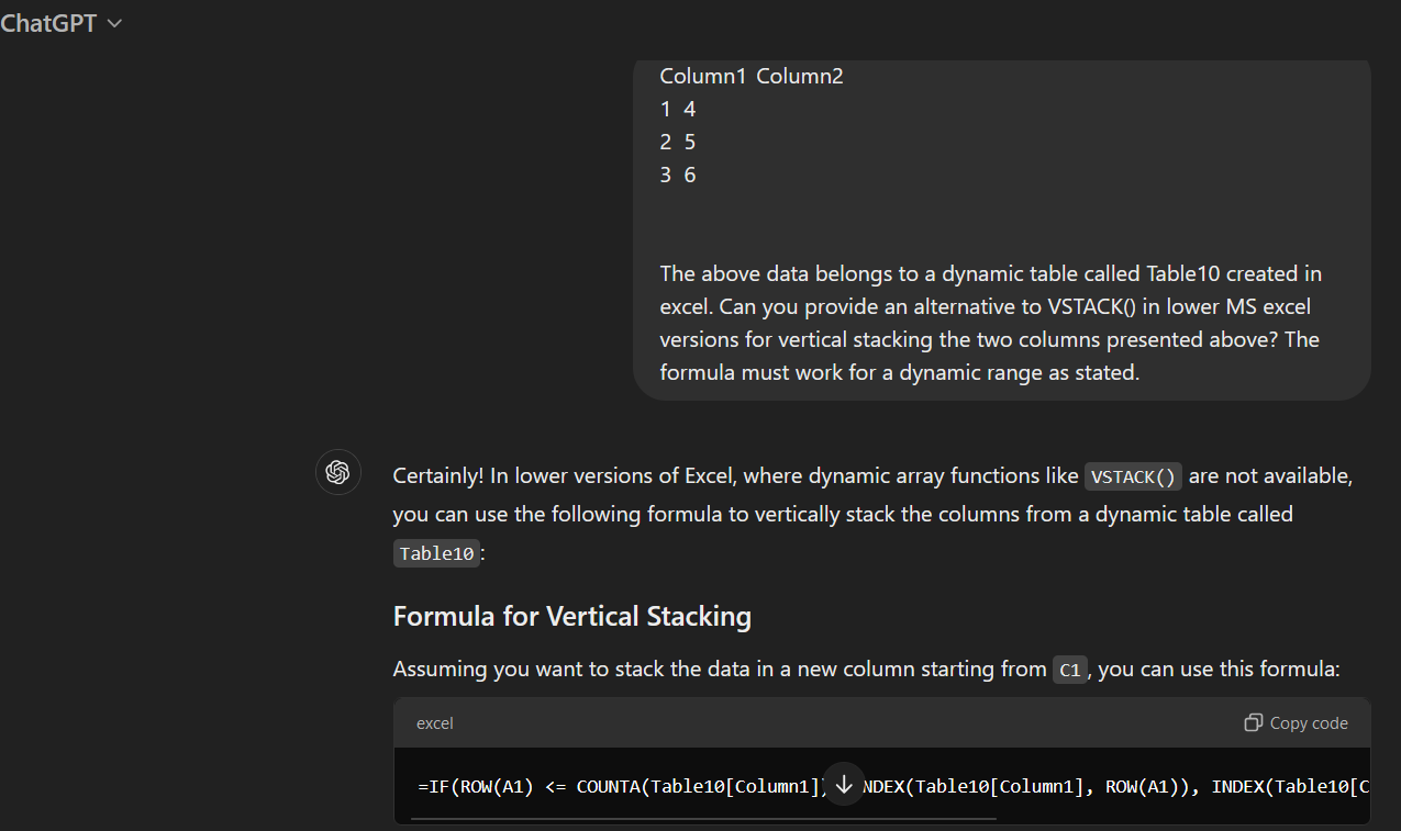
Formula suggested by ChatGPT:
=IFERROR(INDEX(Table10[Column1], ROW(A1)),INDEX(Table10[Column2], ROW(A1)-COUNTA(Table10[Column1])))
Watch the video below to see the Result:
- As you can see here, the formula returned by ChatGPT returned only row and requires you to actually drag the formula down the cells to get the other elements in the stack. This may also cause #!REF error if the range is selected incorrectly.
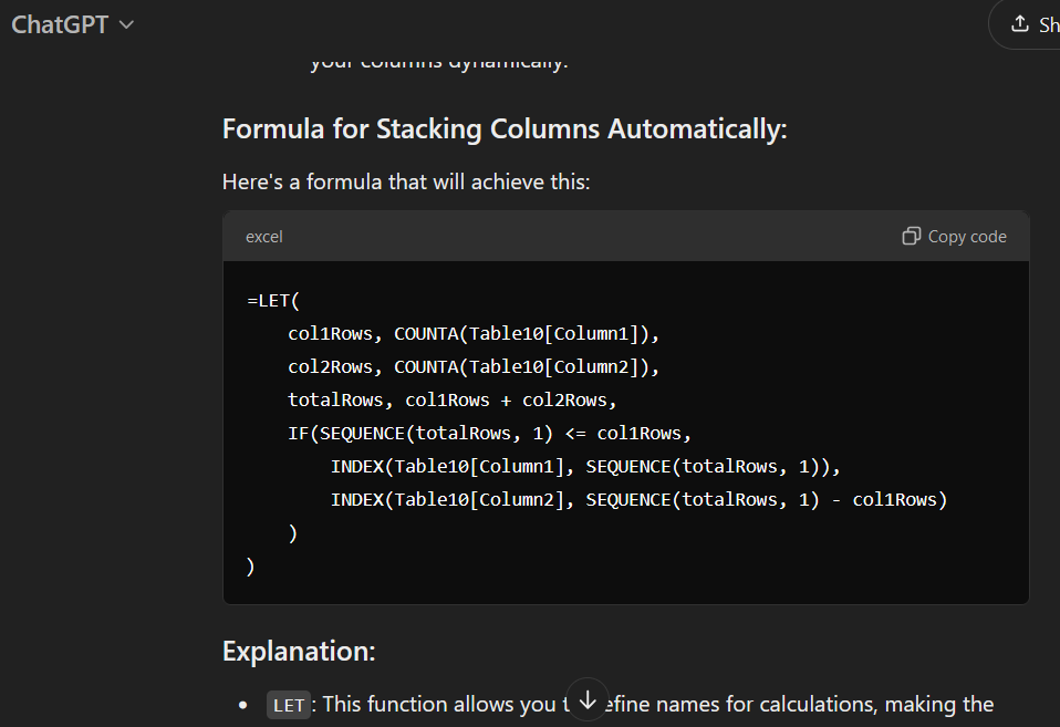
- To resolve this, we asked ChatGPT to optimize the solution to enable dragging automatically using this prompt:
“Can you optimize this formula to automatically drag the formula down to get the complete stack without any human intervention?”
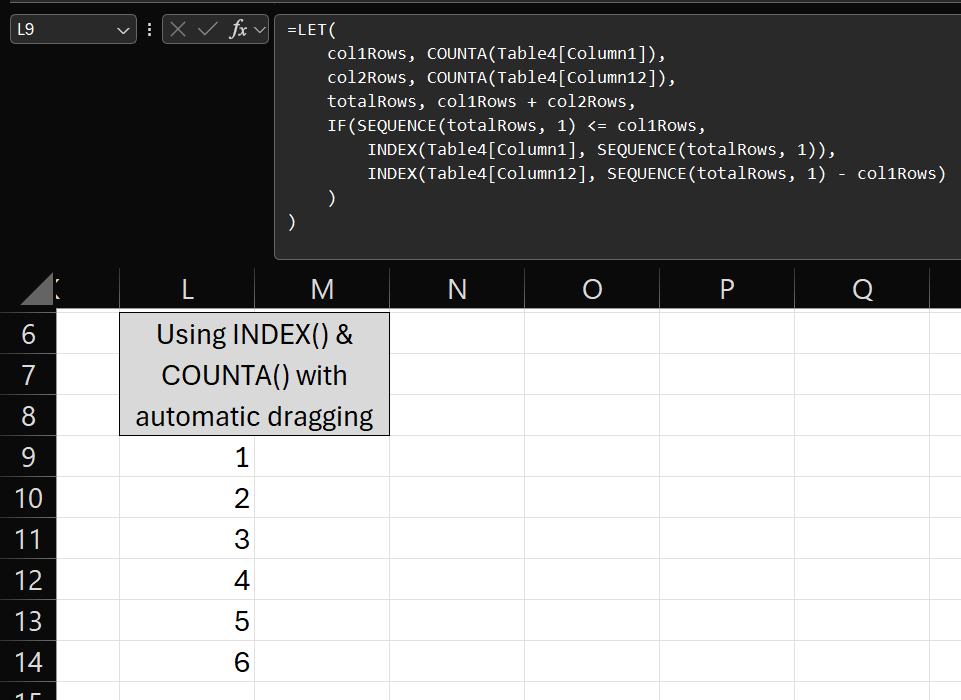
- Here’s the response we got and the associated result:
**
Example 2 : For Horizontal Stacking (HSTACK Equivalent)
- Using INDEX and COLUMN functions:
=INDEX($B$5:$C$7,MOD(COLUMN(C1:H1) – COLUMN(C1), 3) + 1,NT((COLUMN(C1:H1) – COLUMN(C1)) / 3) + 1)
HSTACK() Alternative – Horizontal Stacking with INDEX() and COLUMN()
Explanation of the Formula
- INDEX($B$5:$C$7, …): This specifies the absolute range from which to pull the data.
- MOD(COLUMN(C1:H1)-COLUMN(C1), 3) + 1: This part determines the row number.
- COLUMN(C1:H1)-COLUMN(C1) returns an array of column indices starting from 0 (0, 1, 2, 3, 4, 5).
- MOD(…, 3) gives values from 0 to 2, which corresponds to rows 1, 2, and 3 in the range A1
.
- INT((COLUMN(C1:H1)-COLUMN(C1))/3) + 1: This calculates the column number.
- This portion of the formula determines the column index from B1 and is adjusted to alternate between A and B as you move across the output row.
Using ChatGPT to find Horizontal Stacking Alternative
As we did for vertical stacking alternatives, let’s see what ChatGPT engine has to say about horizontal stacking approaches!
Here’s the prompt we gave to ChatGPT to receive a valid response:
“Write me an alternative to HSTACK() in Excel. The horizontal alignment must be dynamic (without any need to drag the formula across a range of cells). Attached below is the dynamic data table layout. This table is called Table4 and has two columns – Column1 and Column12.”

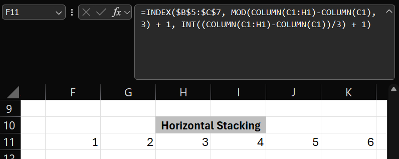
Formula suggested by ChatGPT:
=INDEX(Table4[[Column1]:[Column12]], INT((COLUMN(A1)-1)/2) + 1, MOD(COLUMN(A1)-1, 2) + 1)
Result:

**
4. Troubleshooting Common Issues with VSTACK and HSTACK
Issue 1: Mismatched Array Sizes
When stacking arrays with different sizes, Excel will display #N/A for the missing values.
- Solution: Wrap your VSTACK or HSTACK formula in IFERROR to avoid errors and fill gaps with blank cells.
- =IFERROR(VSTACK(A1:A3, B1:B5), “”)
Issue 2: Dynamic Data Ranges
If your data expands or contracts, fixed cell references may cause issues.
- Solution: Use INDIRECT or INDEX to create dynamic references.
- =VSTACK(INDIRECT(“Sheet1!A2:A”&COUNTA(Sheet1!A:A)))
**
5. VSTACK vs. HSTACK: Key Differences Expanded
Understanding the differences between VSTACK and HSTACK is essential for effective data manipulation in Excel, as they serve distinct purposes based on how you want to arrange your data.
| Aspect | VSTACK (Vertical Stack) | HSTACK (Horizontal Stack) |
| Purpose | Combines multiple ranges into a single vertical array | Combines multiple ranges into a single horizontal array |
| Use Case | Ideal for creating comprehensive lists from different sources | Useful for merging related information into rows |
| Syntax Example | =VSTACK(array1, [array2], …)For ex -=VSTACK(A2:A4, B2:B4, C2:C4) | =HSTACK(array1, [array2], …)For ex -=HSTACK(A2:A4, B2:B4, C2:C4) |
| Data Presentation | Best for vertical lists | Enhances readability by displaying data in rows |
| Dynamic Output | Returns a dynamic array that adjusts with source data changes | Returns a dynamic array that adjusts with source data changes |
| Practical Scenarios | Aggregating survey results or monthly expenses | Summarizing sales data or consolidating project details |
By choosing the appropriate function, you can streamline your workflows and improve data organization in Excel, ultimately enhancing your analytical capabilities.
**
6. Best Practices for Using VSTACK and HSTACK Effectively
- Use Dynamic Ranges: Always reference dynamic ranges to account for changing datasets. You can do so by creating dynamic tables as shown in the examples above.
- Combine with Other Functions: Use FILTER, IFERROR, and SORT for more complex data handling.
7. Frequently Asked Questions (FAQs)
Q1: Can VSTACK and HSTACK be used with other functions?
Yes, they can be combined with other Excel functions like FILTER, SORT, and TEXTJOIN to enhance data manipulation.
Q2: Can I stack data from different sheets?
Yes, VSTACK and HSTACK can handle arrays from different sheets.
8. Conclusion – Stack It Up!
In conclusion, VSTACK and HSTACK are powerful tools in Excel that simplify the way you manage and present data. By understanding how to effectively utilize these functions, you can enhance your productivity and create more organized, readable reports. Whether you need to consolidate lists or merge data from different sources, these dynamic array functions enable you to work efficiently and effectively. We encourage you to experiment with VSTACK and HSTACK in your own projects to unlock their full potential and streamline your data analysis process. Here’s the examples worksheet for you to start your journey: VSTACK and HSTACK examples.xlsx. Happy Excel-ing!