Excel is a tool most commonly used for data analysis, building financial models for efficient decision making. It is used by people with diverse back grounds (i.e; investment bankers, analysts, professionals, students etc.). In excel there are a lot of inbuilt functions which can be used for quick data analysis. In this write up, we will cover 10 most used financial functions in Excel.

1. NPV

Net present value is the present value of cash inflows minus present value of cash outflows. It is used for making capital budgeting/ investment decisions. Decisions could be for an investment in or replacement of a fixed asset, investment or acquisition of a Company or Investment in a Capital-intensive project.

To know more about it, Please refer our blog on Net Present Value

Excel has an inbuilt NPV calculation formula, which calculates the net present value of a series of cash flows at a given discount rate. Negative Cash flows are considered as cash outflows while positive cash flows are considered as cash inflows.

The Syntax for calculating NPV is (rate, Value1, [value2]….)

Rate is the discount rate to be used for discounting the cash flows.

Value1 is the cash flow at the end of Period 1

Value2 is cash flow at the end of Period 2

User has the option to discount up to 254 cash flows using NPV function.

The limitation with NPV function is that excel assumes all the cash flows to occur at the end of the period. Therefore, in for an investment done at the start of the period, add it separately for NPV calculation.

Example

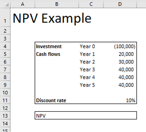
John is considering the financial viability of an investment. The cash flows are as follows.

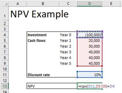
To calculate NPV Type = NPV(rate, cash flows)

= NPV (D11,D5:D9)+D4

We get the NPV of $ 25,185.19 for the investment. That means the investment is acceptable as the present value of cash inflows is greater than present value of cash outflows.

2. XNPV

XNPV is Extended NPV. It measures the NPV of a stream of scheduled cash flows. It is an advance version of NPV. The difference between NPV and XNPV is that in NPV excel cash flows are considered to occur at the end of each period, while in XNPV the cash flows occur at dates defined in the model.

XNPV Syntax

= XNPV(rate, values, dates)

Rateis the discount rate to be applied to the cash flows

Values are the cash flows. Negative cash flows are considered as outflows and positive cash flows are considered as inflows by excel.

Dates are the dates corresponding to the cash flows.

Also Read : Valuation Methodologies for Start-Ups

Important Points

• XNPV does not discount the initial cash flows
• Dates should be in an excel valid format.
• Dates should be in chronological order.
• The range for values and dates should be in sync.

Example

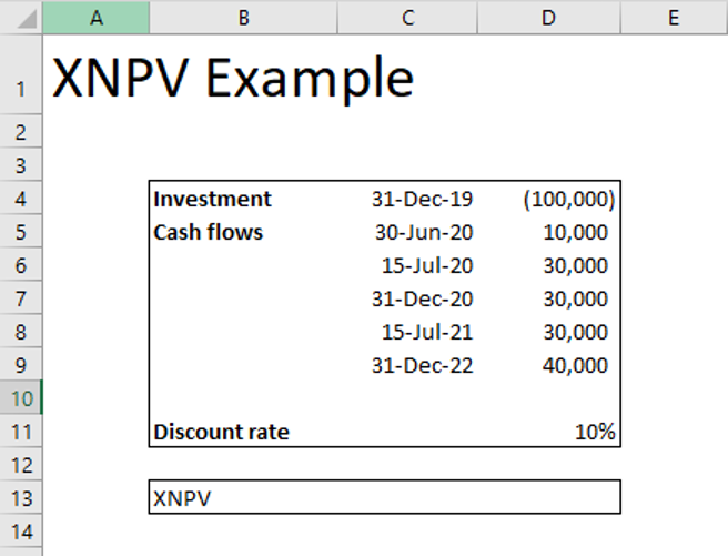
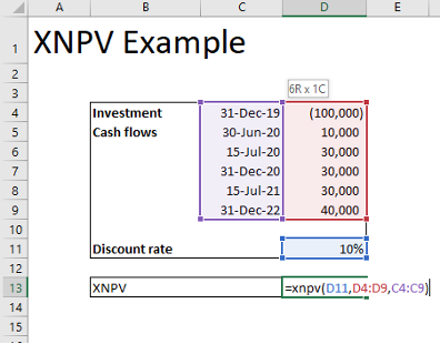
John is considering the financial viability of an investment. The cash flows are as follows. You are required to calculate the XNPV of the cash flows.

To calculate XNPV type = XNPV(rate, values, dates)

= XNPV(D11,D4:D9,C4:C9)

Press Enter. You get XNPV of $21,247.26.

Since XNPV is >0, the investment proposal may be accepted.

3. IRR

IRR is the internal rate of return for a series of cash flows. Internal rate of return is the rate at which present value of cash inflows is equal to the present value of cash outflows (ie, rate at which NPV of the cash flows is Zero). IRR is used to analyze potential investment decisions.

If IRR is greater than cost of capital the project is value creating.

If IRR is less than the cost of capital the project is value destroying.

IRR Syntax

= IRR(Values, [Guess])

Values are the cash flows. It is an array or reference to cells that contain the cash flows. Negative cash flows are considered as outflows and positive cash flows are considered as inflows by excel.

Guess is the number that is close to the result of IRR. It is not mandatory to put the Guess while calculating IRR.

EXAMPLE

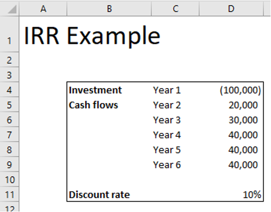
Mr. X is considering the financial viability of an investment. The cash flows are as follows. You are required to calculate the IRR of the investment.

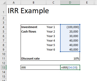
To calculate IRR, type = IRR(Values, [Guess])

= IRR(D4:D9)

Press Enter. You get IRR of 18.37%. Since IRR is greater than the cost of capital. The project can be accepted.

4. XIRR

XIRR also known as Extended internal rate of return is used to calculate the internal rate of return of stream of cash flows occurring during different time period. It is an advance version of the IRR function. It is commonly used while analyzing returns of investments made during different time period.

XIRR Syntax

=XIRR(Values,Dates,[Guess])

Values are the cash flows. It is an array or reference to cells that contain the cash flows. Negative cash flows are considered as outflows and positive cash flows are considered as inflows by excel.

Dates are the dates corresponding to the cash flows.

Guess is the number that is close to the result of IRR. It is not mandatory to put the Guess while calculating XIRR.

Important Points

• XIRR does not discount initial cash flows.
• Dates should be in an excel valid format.
• The range for values and dates should be in sync.

EXAMPLE

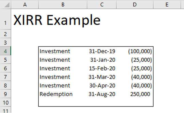
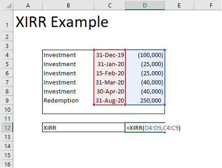
X is investing in a Mutual fund at different time periods. On 31st August 2020, he redeemed all his investments. He wants to calculate the rate of return on his investments.

To calculate XIRR, Type, =XIRR(Values,Dates,[guess])

=XIRR(D4:D9,C4:C9)

Press Enter. You get XIRR of 16.5%.

This means that the return on investment is 16.5% for Mr. X

5. MIRR

Modified internal rate of return or MIRR is a modified version of IRR. IRR is calculated on an assumption that cash flows incurred during the lifetime of a project are reinvested at the internal rate of return. This assumption may not hold true at times.

In Modified IRR the user has the option to enter the financing rate and the reinvestment rate.Thus MIRR solves some of the problems/limitations with IRR.

MIRR Syntax

=MIRR(Values, Finance_rate, Reinvest_rate)

Values is the reference to series of cash flows from a project. Negative cash flows are considered as cash outflows, while positive cash flows are considered as cash inflows.

Finance_rateis the interest rate paid on the investment.

Reinvest_rate is the interest rate received on cash flow which are reinvested.

EXAMPLE

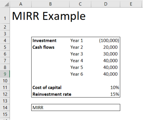
Mr. X is considering the financial viability of an investment. The cash flows are as follows. You are required to calculate the MIRR of the investment.

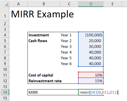
To calculate MIRR, type = MIRR(Values,finance_rate,Reinvest_rate)

=MIRR(D4:D9,D11,D12)

MIRR = 17%, means that the modified internal rate of return from the investment is 17%, which is well above the cost of capital. Hence the project/investment can be accepted

Read our blog on How to Calculate Weighted Average Cost of Capital

6. PMT

The PMT or payment function helps calculate the loan EMI.

PMT SYNTAX

=PMT(rate,nper,PV,[FV],[type])

Rate is the interest rate for the loan.

Nper is the total no. of instalments.

PV is the present value of the loan

FV is the future value of the loan after the last payment is made.

Type is the logical value; you should enter 1 if the EMI payment is at the beginning of the period, or 0 if the EMI payment is at the end of the period. You can also leave it blank. In that case it will be considered as 0 by excel.

EXAMPLE

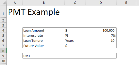
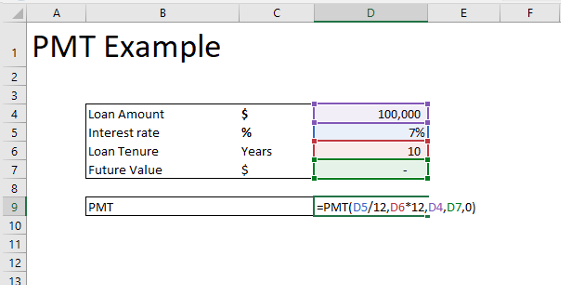
Mr. K is considering to take a home loan of $100,000 for 10 years. The interest rate is 7%. He wants to know the EMI on the loan amount.

To calculate the EMI type, = PMT(rate,nper,PV,FV,Type)

=PMT(D5/12,D6*12,D4,D7,0)

Press Enter. You get PMT of $1,161,08.

This means that Mr. K would have to pay $1,161.08 for 10 years (ie, 120 months) to repay the loan amount.

7. NPER

NPER calculates the number of periodic payments (instalments) to be made if the rate of interest remains constant and the opening and closing balances are known.

This is generally used to calculate the Tenure of the Loan EMI, if the interest rate, Principal loan amount and outstanding balance at the end of the period and monthly payment is known.

NPER SYNTAX

=Nper(Rate,PMT,PV,[FV],Type)

Rate is the interest rate for the loan.

PMT is the periodic cash outflow.

PV is the present value of the loan

FV is the future value of the loan after the last payment is made.

Type is the logical value; you should enter 1 if the EMI payment is at the beginning of the period, or 0 if the EMI payment is at the end of the period. You can also leave it blank. In that case it will be considered as 0 by excel.

EXAMPLE

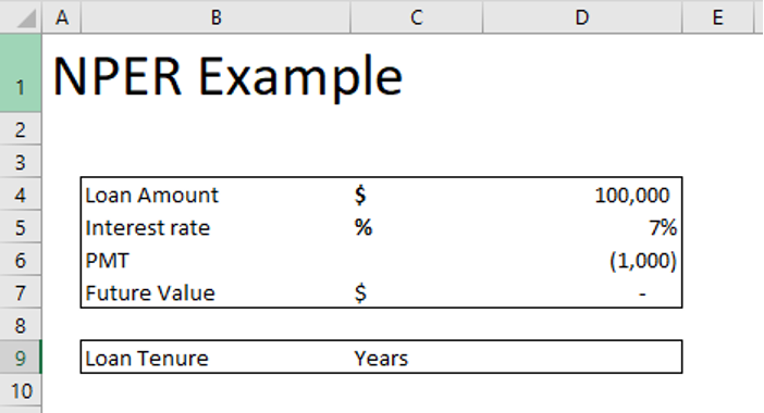
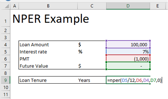
Mr. K is considering to take a home loan of $100,000. The interest rate is 7%. He can pay $1000 as EMI. What will be the loan Tenure.

To calculate the period of instalments type, =Nper(Rate,PMT,PV,[FV],Type)

=Nper(D5/12,D6,D4,D7,0)

NPER = 150.52 months

When you divide it by 12, you get 12.54 years.

That means that you will have to pay $1000 for 12.54 years to repay the loan amount of $100,000, if the interest rate remains constant at 7%.

8. RATE

Rate function calculates the rate of interest on the loan or investment.

RATE SYNTAX

=Rate(NPER,PMT,PV,[FV],[Type])

NPER is the total no. of instalments.

PMT is the periodic payment made. This amount remains constant during the tenure of the loan or investment.

PV is the present value of the loan

FV is the future value of the loan after the last payment is made.

Type is the logical value; you should enter 1 if the EMI payment is at the beginning of the period, or 0 if the EMI payment is at the end of the period. You can also leave it blank. In that case it will be considered as 0 by excel.

EXAMPLE

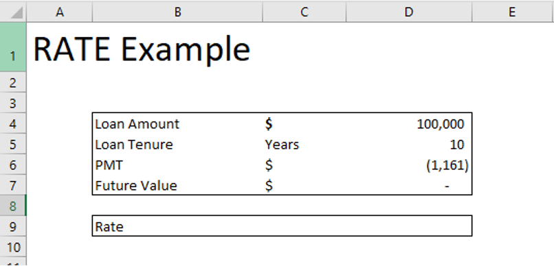
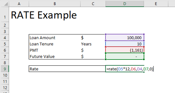
John is considering taking a home loan of $100,000. He has been asked to pay an EMI of $1,161 for 10 years. What is the interest rate on the loan?

To calculate the rate, type =rate(NPER,PMT,PV,[FV],[Type])

=Rate(D5*12,D6,D4,D7,0)

Press Enter. You get Rate of 0.58%. This is the monthly rate. When you multiply it by 12, you get 7%. This is the annual rate of interest on the loan or investment.

9. PPMT

PPMT function returns the principal payment for a given loan based on periodic constant payments and constant interest rate.

PPMT Syntax

= PPMT(Rate, Per, Nper, PV, [FV],[Type])

Rate is the interest rate for the loan.

Per specifies the period and must be between 1 and NPER.

NPER is the total no. of instalments.

PV is the present value of the loan

FV is the future value of the loan after the last payment is made.

Type is the logical value; you should enter 1 if the EMI payment is at the beginning of the period, or 0 if the EMI payment is at the end of the period. You can also leave it blank. In that case it will be considered as 0 by excel.

EXAMPLE

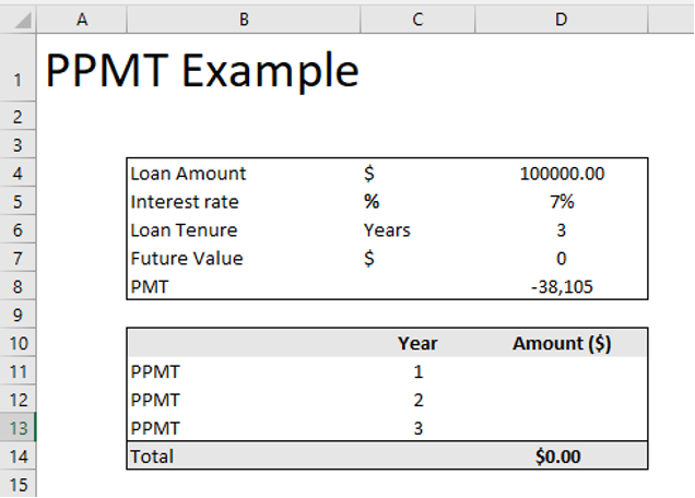
X is taking a loan of $100,000 at 7% interest per annum. He wants to repay it in 3 equal yearly. Instalments. The annual payment is $38,105 Calculate the Principal repayment in year 1, 2 and 3.

To calculate the PPMT, type = PPMT(Rate, Per, Nper, PV, [FV],[Type])

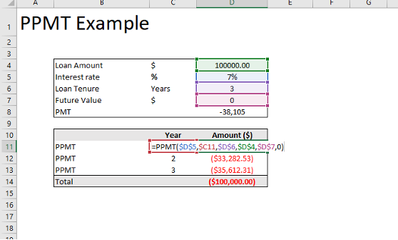
=PPMT($D$5,$C11,$D$6,$D$4,$D$7,0)

Press Enter. You get $31,105.17 as Principal payment for year 1.

If you Copy and Paste this formula to cells D12 and D13, you get the principal payment for year 2 and 3 as well.

10. IPMT

IPMT function returns the interest payment for a given loan based on periodic constant payments and constant interest rate.

IPMT SYNTAX

=IPMT(Rate,Per,Nper,PV,[FV],[Type])

Rate is the interest rate for the loan.

Per specifies the period and must be between 1 and NPER.

NPER is the total no. of instalments.

PV is the present value of the loan

FV is the future value of the loan after the last payment is made.

Type is the logical value; you should enter 1 if the EMI payment is at the beginning of the period, or 0 if the EMI payment is at the end of the period. You can also leave it blank. In that case it will be considered as 0 by excel.

EXAMPLE

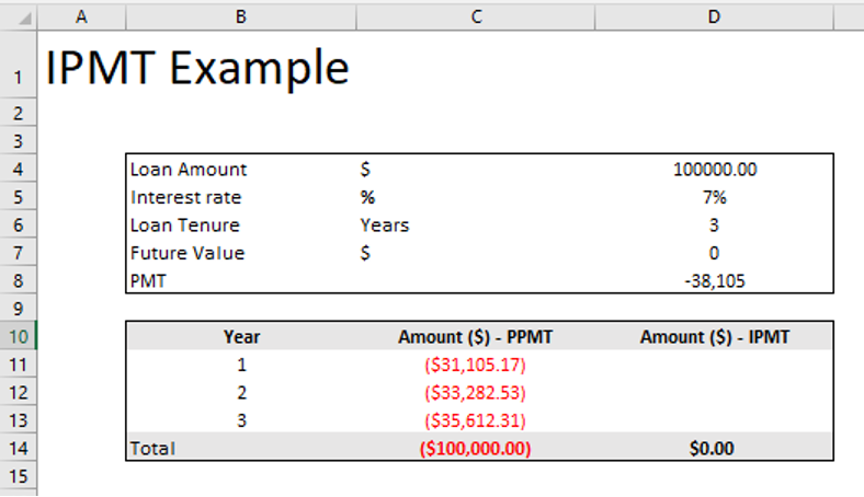
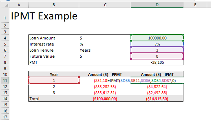
Taking the Previous Example. X is taking a loan of $100,000 at 7% interest per annum. He wants to repay it in 3 equal yearly Instalments. The annual payment is $38,105. Calculate the Interest repayment in year 1, 2 and 3.

To Calculate IPMT type, = IPMT(Rate,Per,Nper,PV,[FV],[Type])

=IPMT($D$5,$B11,$D$6,$D$4,$D$7,0)

Press Enter. You get IPMT of $7,000/- for Year 1.

If you Copy and Paste this formula to cells D12 and D13, you get the Interest payment for year 2 and 3 as well.

Note that total PPMT and IPMT is Equal to PMT which is $38,105 as calculated above.

Let us know if you have any questions/ comments by posting in the comments section. There is also an Excel cheat sheet compilation that can help to remember some of the formulas.

You can also learn more about this blog on our LinkedIn page as well 🙂