Imagine you’re an investor eyeing a call option on Tesla’s stock, wondering if it’s worth buying today. How do you figure out the appropriate price to offer? This is where an option pricing model steps in, serving as the backbone of financial decision-making by quantifying the value of stock options and derivatives. These models blend mathematics, statistics, and market dynamics to calculate fair prices, empowering investors to navigate the complexities of modern markets.
WHAT IS AN OPTION PRICING MODEL?
Option pricing models are mathematical frameworks used to estimate the value of an option. They consider factors like the underlying asset’s current price, the strike price, time to expiration, volatility, interest rates, and potential dividends. Accurate pricing is crucial because it helps traders and companies hedge risks, strategize on investments, and optimize returns.
WHAT IS AN OPTION?
An option is a financial contract that gives you the right, but not the obligation, to buy or sell an asset (like a stock) at a specific price, called the strike price, within a certain time period. There are mainly two types of options:
- Call Option (C): Gives you the right to buy an asset at the strike price. For instance, if Tesla’s stock is valued at $100 and you own a call option with a strike price of $90, you have the opportunity to purchase the stock at $90, resulting in a $10 profit per share if the market price remains above $90.
- Put Option (P): Gives you the right to sell an asset at the strike price. Example: If Tesla’s stock drops to $80, and you have a put option with a strike price of $90, you can sell the stock for $90, earning $10 per share above the market price.
Options can also be categorized based on when they can be exercised as follows:
- European Options: These can only be exercised on their expiration date. Example: If you hold a European call option expiring on June 30th, you can only buy the underlying asset on that day, not before.
- American Options: American options can be exercised at any point before their expiration date.
Think of an Option like a Reservation. You pay a small fee upfront (called the premium) for this right. If the deal is favorable, you can exercise your option. If not, you can let it expire, losing only the paid premium.
Options are powerful tools for traders and investors, helping them profit from price movements or manage risks without owning the underlying asset directly.
HOW DO WE KNOW WHEN TO EXERCISE THE OPTION?
In options trading, the terms In the Money (ITM), At the Money (ATM), and Out of the Money (OTM) describe an option’s profitability based on the strike price and the underlying asset’s current price. ITM options are profitable to exercise; for call options, this means the asset price is above the strike price, while for puts, it’s below. OTM options would result in a loss if exercised since the asset price is below the strike price for calls or above it for puts. ATM options have a strike price close to the asset’s current price, offering no immediate profit but high sensitivity to market movements.
| Term | Call Option | Put Option | Profitability |
| In the Money | Asset price > Strike price | Asset price < Strike price | Profitable to exercise |
| At the Money | Asset price ≈ Strike price | Asset price ≈ Strike price | No profit; highly sensitive |
| Out of the Money | Asset price < Strike price | Asset price > Strike price | Not profitable to exercise |
WAYS TO VALUE OPTIONS
Option valuation methods, such as the Black-Scholes Model and the Binomial Model, help determine the fair price of options by analyzing factors like the stock price, strike price, time to maturity, volatility, and risk-free interest rates. While the Black-Scholes Model offers a continuous framework for European options, the Binomial Model uses a step-by-step tree approach, making it flexible for both American and European options.
WHAT IS RISK-NEUTRAL PROBABILITY IN OPTION PRICING MODEL?
Before delving into various option pricing models, it’s important to understand the concept of risk-neutral probabilities, which play a key role in many of these models.
A risk-neutral probability is a theoretical probability that adjusts for risk, and it reflects the likelihood of different outcomes in an idealized market. The concept rests on two key assumptions:
- The current price of an asset is equal to its expected future payoff, discounted at the risk-free rate.
- There are no arbitrage opportunities in the market, meaning there are no risk-free profits to be made.
It’s important to note that we do not assume that all investors are actually risk-neutral, nor that risky assets will earn the risk-free rate of return. Instead, the risk-neutral probability serves as a theoretical construct to model asset pricing under ideal conditions, assuming a simplified world where all assets are priced according to a single, unified probability distribution.
Let’s understand this with the help of an example. Let’s assume there is a stock priced today $50 and there are only two possibilities: the stock price can either move 20% up ($60) or 20% down ($40) over a period of 1 year. If relevant risk free rate in this time period is 4%, then risk neutral probability is that probability that will give us an expected payoff equal to 4%. By simple hit and trial method we can figure out that if there is 60% probability of up move and 40% probability of down move, then the expected payoff will be 4%.
Expected Payoff Calculation:
Expected Payoff= 60% * ($60/$50-1) + 40%*($40/$50-1)
= 60%*20%+40%*-20%
= 12%-8%
=4%
If we had an option with strike price of $50 for the same stock the price of the option using these risk neutral probability (60% up and 40% down) would be calculated as:
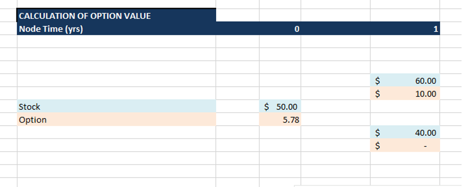
Option Payoff at Maturity= 60%*$10+40%*0 = $6
Option value today= Present value of $6 (discounted at 4%) = $5.78
BINOMIAL OPTION PRICING MODEL
The Binomial Option Pricing Model estimates the fair value of an option by modeling potential future stock prices as a decision tree with discrete time steps. At each step, the stock can move up or down by certain factors, creating a lattice of possible prices. The model then calculates the option value backward from the expiration date, considering probabilities and the time value of money.
Main Assumptions of the Model:
- The stock price follows a binomial distribution with two possible movements per time step (up or down).
- The market is arbitrage-free, meaning there’s no guaranteed risk-free profit.
- Investors can borrow or lend at a risk-free rate like treasury bills.
- The option can only be exercised at its maturity date, which is a characteristic of European options.
Let’s understand how to calculate the call option and put option values using the simple example below.
| Assumptions | |
| Stock price today (S) | $ 50.00 |
| Strike price (K) | $ 55.00 |
| Step | 1 |
| Time to Maturity (T) | 1 year |
| Risk-free interest rate (r ) | 5% |
| Volatility (σ) | 20% |
| Time/Step ∆t | 1 |
Step 1: Define Up and Down Factors
u = 1/d
Up factor (u) =
Down factor (d) = 1/u = 1/1.2214 = 0.8187
The up and down factors represent the potential price movements of the stock. An up factor (u) of 1.2214 means the stock could increase by 20%, while a down factor (d) of 0.8187 means it could decrease by 20%. The relationship of u=1/d ensures consistency in price changes.
Step 2: Calculate Stock price upward and downward
Possible future prices are determined by multiplying the current price by u and d.
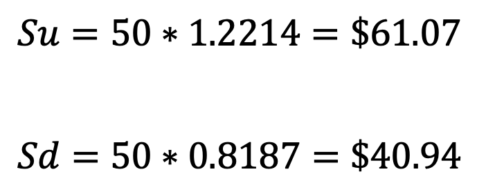
Step 3: Calculate Risk-Neutral Probability (p)
This adjusts the probability of stock movements to a risk-free world where expected returns equal the risk-free rate. Using the formula p =
pu = (1.0513 – 0.8187)/ (1.2214 – 0.8187) = 0.5775
Note: In Excel,
P is the probability of the stock moving upward. To find the movement of stock downward we shall take probability as 1-p i.e.,
Pd= 1-Pu = 1- 0.5775 = 0.4225
Step 4: Calculate Option Payoff at Maturity
For a call option, the payoff is:
Max
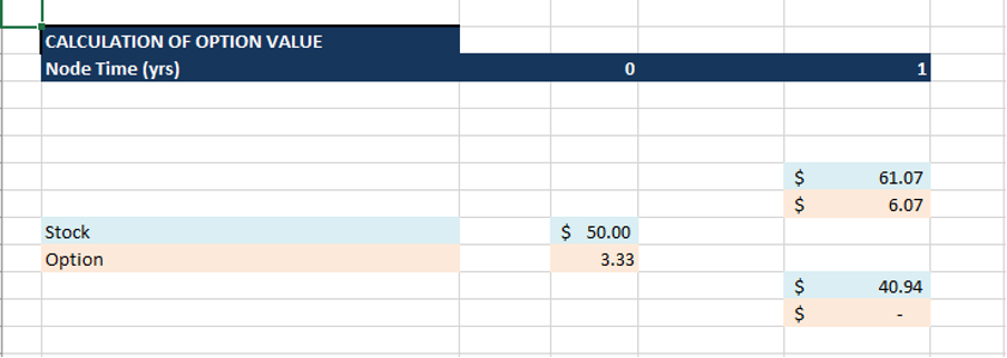
Up move payoff = max (61.07 – 55,0) = 6.07
Down move payoff = max (40.94 – 55, 0) = 0
For a put option, the payoff is:
Max
Up move payoff = max (55 – 61.07, 0) = 0
Down move payoff = max (55 – 40.94, 0) = 14.06
Step 5: Discount Back to Today
The option’s current value combines the expected payoff and the time value of money. We can calculate the Call Option value as below.

= 0.9512 * [ 0.5775 * 6.07 + 0.4225 * 0]
= 0.9512 * [3.51 + 0]
= $3.33
We can calculate the Put Option value as below.

= 0.9512 * [ 0.5775 * 0 + 0.4225 * 14.06]
= 0.9512 * [0 + 5.94]
= $5.65
Note:
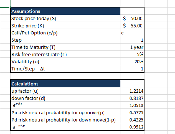
We have calculated the same example in the Excel workbook for your ready reference as below. Download the Excel file to practice with your numbers. Also, the workbook contains an example with a 3-step and 5-step binomial model.
Call Options Calculation in Excel
Put Options Calculation in Excel
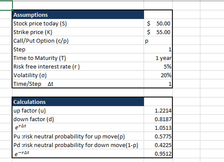
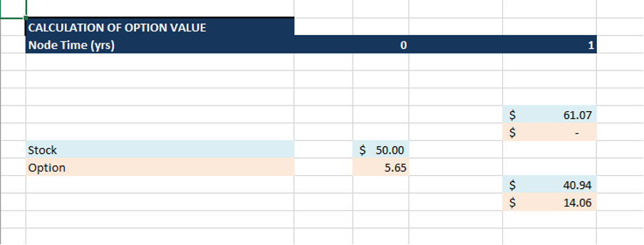
BLACK-SCHOLES OPTION PRICING MODEL
The Black-Scholes Model is a widely used mathematical formula for valuing European options, which can only be exercised at maturity. It estimates the fair price of a call or put option by accounting for factors like the current stock price, strike price, time to maturity, volatility, and the risk-free interest rate.
Main Assumptions of the Model:
- The underlying stock does not distribute any dividends during options life.
- Markets operate without arbitrage opportunities, meaning no risk-free profit.
- The stock price has constant volatility over time.
- Stock prices follow a lognormal distribution.
- Stocks can be traded at any time without restrictions.
- The risk-free interest rate remains constant during the option’s life.
FORMULA FOR CALCULATION OF OPTION VALUE USING BLACK SCHOLES MODEL
The Black-Scholes formula for a European call option is:

The Black-Scholes formula for a European put option is:

Where,


N(d) = Cumulative probability under a standard normal distribution.
Let’s understand how to calculate the call option and put option values using the simple example below.
| Assumptions | |
| Stock price today (S) | $ 50.00 |
| Strike price (K) | $ 55.00 |
| Time to Maturity (T) | 1 year |
| Risk-free interest rate (r ) | 5% |
| Volatility (σ) | 20% |
Step 1: Calculate d1 and d2
These values represent the probabilities under a risk-neutral world that the stock price will exceed the strike price at expiration. They are adjusted by volatility and time.
- d1: Reflects the adjusted probability that the stock price will exceed the strike price K.
- d2: Derived by subtracting
Formula,

= ln(50/55) + [5% + (20% ^ 2)/2] * 1
20%* SQRT(1)
=-0.1266

= -0.1266 – [20% * SQRT (1)]
= -0.3266
Step 2: Find N(d1) and N(d2) for call option and N(-d1) and N(-d2) for put option
N(d1): The cumulative probability that the stock price exceeds the strike price 𝐾 at expiration.
N(d2): Represents the risk-neutral probability that the option will be exercised.
These values come from the standard normal distribution, which models the likelihood of different outcomes. N(d1) is higher than N(d2)because it accounts for the expected growth of the stock.
A negative d1 and d2 flips the probabilities since they refer to the stock price being below the strike price for a put option.
In the Excel, we can calculate N(d1) and N(d2) using NORM. S. DIST function.
In our example
N(d1) = NORM.S.DIST (-0.1266, True) = 0.4496
N(d2)= NORM.S.DIST (-0.3266, True) = 0.3720
N(-d1) = NORM.S.DIST (-(-0.1266), True) = 0.5504
N(-d2)= NORM.S.DIST (-(-0.3266), True) = 0.6280
Step 3: Calculate the Stock Price component
For the Call Option, the Stock Price component is calculated as S0.N(d1). It represents the weighted value of the stock price adjusted by the probability N(d1) that the option will finish in the money (stock price > strike price).
S0.N(d1)= $50 * 0.4496 = $22.48
For the Put Option, the Stock Price component is calculated as S0.N(-d1). It represents the weighted value of the stock price adjusted by the probability N(d1), that the option will not finish in the money (stock price <= strike price).
S0.N(-d1)= $50 * 0.5504 = $27.52
Step 4: Calculate the Strike Price component
For the Call Option, the Strike Price component is calculated as K.e-rt.N(d2) It represents the discounted strike price, weighted by the probability N(d2) that the call option will be exercised (stock price > strike price). It reflects the cost of paying the strike price if the option is in the money at maturity.
K.e-rt.N(d2) = $55 * 0.9512 * 0.3720 = $19.46
For the Put Option, the Strike Price component is calculated as K.e-rt.N(-d2). It represents the discounted strike price, weighted by the probability N(-d2)that the put option will be exercised (stock price < = strike price). It reflects the benefit of receiving the strike price if the option finishes in the money.
K.e-rt.N(-d2)= $55 * 0.9512 * 0.6280 = $32.86
Step 5: Calculate the Option Value
For the Call option, subtract the Strike Price Component from the Stock Price Componet
C= S0.N(d1) – K.e-rt.N(d2)
= $22.48 – $19.46
= $3.02
For the Put option, subtract the Stock Price Component from the Strike Price Component
P= S0.N(-d1) – K.e-rt.N(-d2)
= $32.86 – $27.52
= $5.34
We have calculated the same example in the Excel workbook for your ready reference as below. Download the Excel file to practice with your numbers.
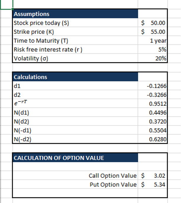
WHY DO THE OPTION VALUES VARIES FROM THE BINOMIAL AND BLACK SCHOLES MODEL DISCUSSED ABOVE?
The difference between the results of the Binomial Pricing Model and the Black-Scholes Model stems from the distinct approaches these models use to calculate option values. The Black-Scholes Model assumes continuous stock price movement and provides a formula-based solution, while the Binomial Model uses discrete time steps, simulating stock price changes in up or down movements at each step. These methodological differences can lead to variations in option values. However, the difference can be minimized by increasing the number of time steps in the Binomial Model, as this allows it to closely approximate continuous stock price behavior, aligning more closely with the assumptions of the Black-Scholes framework.
For instance, in our example above we get the following results for call and put options under both the methods for 1 year and 1 step model.
| Model Type | Call | Put |
| Binomial | $ 3.33 | $ 5.65 |
| Black Scholes | $ 3.02 | $ 5.34 |
From the above table, we can see that there is a very small difference between the option values from both models.
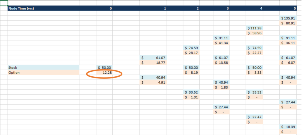
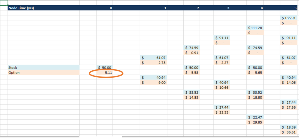
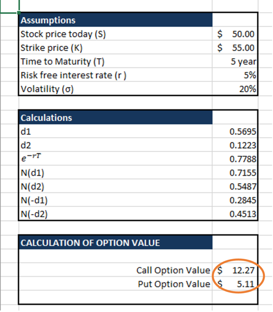
However, if we build a binomial model with the assumption of 5 years and 5 steps (remaining assumptions remaining same as above) and the Black Scholes model with 5 years as an assumption (rest of the assumptions being the same as above), we get the following option values.
| Model Type | Call | Put |
| Binomial | $ 12.28 | $ 5.11 |
| Black Scholes | $ 12.27 | $ 5.11 |
From the above table, it is proved that if we increase the steps in the Binomial model we will get results close to the Black Scholes model. The Excel calculations for the same is shown below.
Call option calculated by Binomial option pricing model
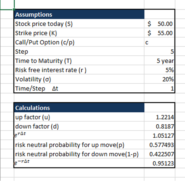
Put option calculated by Binomial option pricing model.
Call and Put option calculated by Black Scholes model.
PROS AND CONS OF OPTION PRICING MODEL
| Aspect | Binomial Pricing Model | Black-Scholes Model |
| Pros | ||
| Flexibility | Handles a variety of option types, including American options (which can be exercised at any time before expiration). | Suitable for European options with continuous-time assumptions. |
| Simplicity in assumptions | Incorporates discrete time intervals, making it easier to understand intuitively complex scenarios. | Assumes continuous time and provides a closed-form solution for quick and efficient computation. |
| Customization | Can model varying volatility or interest rates over time. | Applicable to standard market assumptions with constant volatility and interest rates. |
| Cons | ||
| Computational intensity | Requires significant time and resources for a large number of steps to achieve high accuracy. | Limited to options with standard assumptions, such as constant volatility and European exercise style. |
| Complexity for extensions | Becomes more complex when adapting for stochastic interest rates or dividend-paying stocks. | Cannot handle American options or scenarios with non-standard conditions. |
| Accuracy in discrete steps | May produce less precise results for fewer steps compared to continuous models. | Relies on idealized assumptions that may not hold in real-world markets, such as log-normal price distribution. |
CONCLUSION
An Option pricing model, such as the Binomial Model and Black-Scholes, are essential tools that blend probability, risk, and time to help investors navigate financial markets. The Binomial Model offers flexibility by simulating price changes step-by-step, while the Black-Scholes formula provides a concise solution for European options. Both models reveal how factors like volatility, time, and dividends influence option values, enabling strategic decision-making in uncertain markets. Mastering these models empowers investors to make informed, calculated bets on the future, turning complex market dynamics into actionable insights.


