WHAT IS EXCEL OFFSET FUNCTION?

Offset function returns a reference to a range that is a given number of rows and columns from a given reference. This reference point in the Offset formula is the starting cell supplied as an argument to the function and beginning from this reference point, the offset function works out an ending cell or range whose value is returned.

Syntax of the function is as follows:

OFFSET (reference, rows, cols, [height], [width])

Where,

• Reference (required)- is the reference from which we want to base the offset, a reference to a cell or range of adjacent cells. We can think it of as the starting point.
• Rows (required)- is the number of rows up or down, that we want the upper-left cell of the result to refer to. Basically, it is the number of rows up or down to move from the starting point, i.e., the reference point. If the row number is positive, then the formula moves below the starting reference and in case of a negative number the formula goes above the starting reference.
• Cols (required)- is the number of columns, to the left or right, that we want the upper-left cell of the result to refer to. Basically, it is the number of columns up or down to move from the starting point, i.e., the reference point. If the column number is positive, then the formula moves to the right of the starting reference and in case of a negative number the formula goes to the left of the starting reference.
• Height (optional)- is the height, in the number of rows, that we want the result to be, the same height as reference if omitted.
• Width (optional)- is the width, in number of columns, that we want the result to be, the same width as Reference if omitted.

Points to be noted:

1. The height and width arguments both must always be positive numbers.
2. If either height or width is omitted, it defaults to the height or width of reference.
3. The Offset function is volatile and may slow down the excel worksheet in which it is used. The slowness of the worksheet is directly proportional to the number of cells recalculated.
4. The first three arguments i.e., the reference, rows and cols are required and the last two arguments are optional.
5. In actual any cells or range are not moved by the Offset function in excel. The function just returns a reference.
6. The rows and cols arguments in the Offset function always refer to the upper-left cell in the returned rage, when the Offset function returns a range of cells.
7. The Offset formula will return the #VALUE! Error if the reference argument does not include a cell or range of adjacent cells.
8. The OFFSET formula will return the #REF! error in case the specified rows and/or cols move a reference over the edge of the spreadsheet.

REASONS FOR USING THE EXCEL OFFSET FUNCTION

Following are the reasons to use the offset function in excel:

1. The function helps to find the value of a cell or range whose starting point is known but whose address is unknown.
2. The function works with data set in which rows or columns are added regularly.
3. The function helps to create a dynamic range for PivotCharts and Pivot Tables.
4. This function can be combined with other excel functions like sum, average, max, min etc., which require the cell address to work.
5. It is a good alternative to the VLOOKUP function since it does not require data to be in a set format for data analysis.

BASIC EXAMPLE of EXCEL OFFSET

Let us understand the Offset function with the help of a very simple example where the function returns a cell reference based on the starting point, rows and columns that we specify in the formula.

The Offset function is written as

=OFFSET(A1,4,1)

The offset function tells the excel to move cell A1 (the reference point
) 4 rows down (row argument) and one column to the right (cols argument). As a result, the function returns value in cell B5.

Below we have shown the route the function follows:

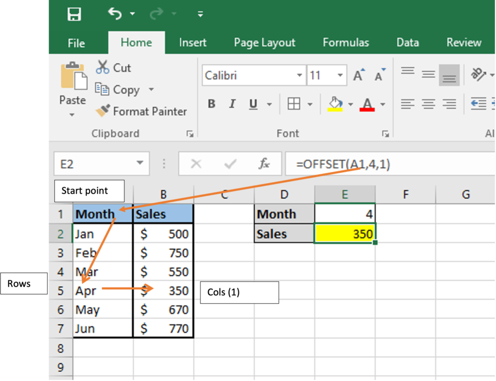
In the above formula we can also use cell reference in place of rows argument as follows and we will get the same result:

=OFFSET (A1, E1,1)

IMPORTANT: If we want the Offset function to return a range as a result in versions older than excel 365 we can use F9 key to check results returned from OFFSET.

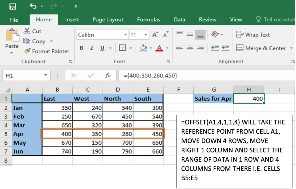
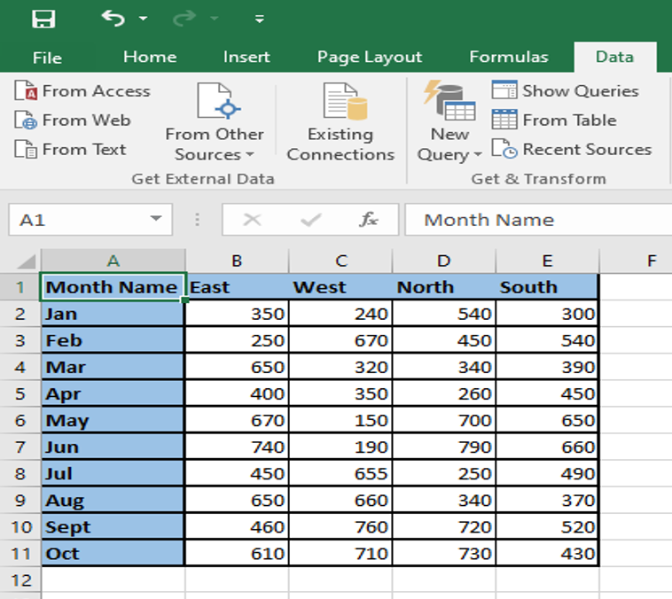
Example: We have list of sales of a company month wise and region wise. We want to find sales for the April month for all the regions. We will use the below syntax to get the results.

When we enter the syntax =OFFSET(A1,4,1,1,4), we get #VALUE! Error, since we are using the EXCEL version below excel 365. We can however view the result using the F9 key. We need to press F9 when entering the syntax =OFFSET(A1,4,1,1,4). The result can be viewed in the formula bar and not a single excel cell. In the above formula the height is 1 and width is 4.

BASIC EXCEL OFFSET AND SUM FUNCTIONS

We can use the Offset function along with other excel functions. Let us first understand how Offset can be used along with the SUM function.

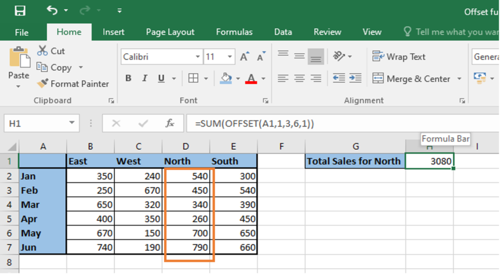
Example: Taking the above example of sales month wise and region wise we want to get sum of total sales in the North region for all the months from Jan to Jun. We will use the below syntax.

=SUM(OFFSET(A1,1,3,6,1))

A DYNAMIC SUM WITH EXCEL OFFSET FORMULA

In real life we usually work with worksheets that keeps being updated continuously. In such cases we need a sum formula that automatically sums up the newly added rows or columns. Suppose in the above example we have new rows added every month with the month name and we want the sum total to include the newly added rows as well, we can either update the range in the SUM formula manually or let the Offset function do the same for us.

We want a formula that gives us the sum total of Sales for the North region for all the months including the new month being added.

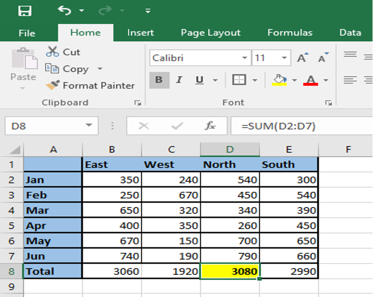
At present the total sales for North region from Jan to June is $3,080.

Suppose you add a new row with July data as well. Now, to get the sales for North region from Jan to July we will use the below syntax.

=SUM(D2:OFFSET(D9,-1,0))

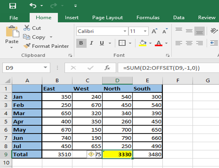
The first cell of the range to the SUM function will remain the same. However, the second cell to the range will keep changing constantly and hence we use Offset function here to make the sum function more dynamic. Here in the Offset function,

• Reference: shall be the cell containing the total, in this case the reference being cell D9.
• Rows: shall be the cell right above the total and hence since we are moving upwards the reference we will use the negative sign i.e., -1.
• Cols: shall be 0 because we want sales for the same column i.e., the North region.

Hence, the syntax to be used shall be

=SUM(first cell:(OFFSET(cell with total, -1,0)

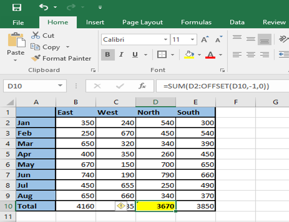
If we further add the August month data as a new row, the total will automatically get updated as below

EXCEL OFFSET FORMULA TO SUM THE LAST N ROWS

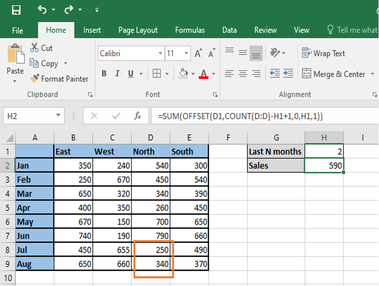
Instead of getting the sum total of sales for the entire North region, suppose we want the total of sales for the last N months and also want the formula to include automatically any new rows that we add to the table above, we will use the offset function in combination with the SUM and COUNT/COUNTA functions.

For example, we want to know the total sales for the newly added July and August months, we will use the below syntax.

=SUM(OFFSET(D1,COUNT(D:D)-H1+1,0,H1,1))

Or,

Where,

• Reference: the column header whose values we want to sum, here it is D1
• Rows: we can use either the COUNT or COUNTA function to calculate the number of rows to offset. COUNT function returns the number of cells in column D that contain numbers, from which we subtract the last N months (the number is cell H1), and add 1.

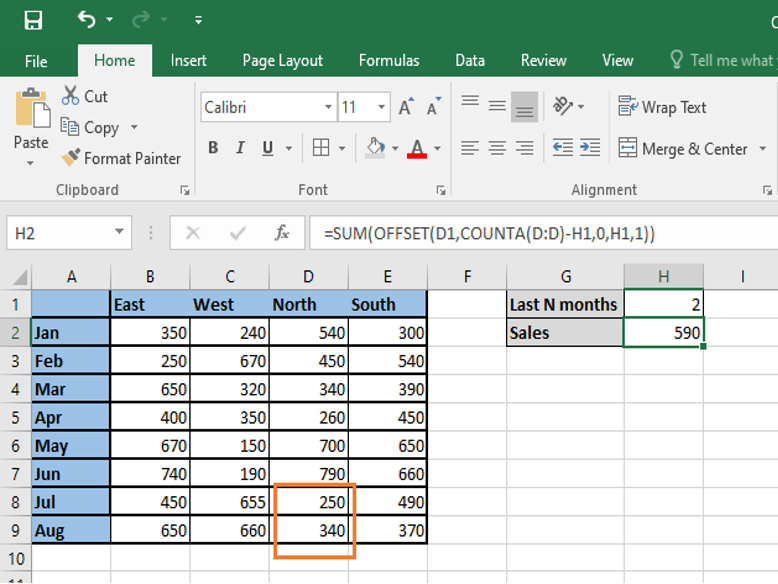
In case we use COUNTA function we do not need to add 1. This function counts all non-empty cells and a header row with a text value adds an extra cell in the formula and hence no need to add 1 separately.

• Cols: Since we want to stay in the same column, we will use 0 here.
• Height: the number of rows whose sum is required is specified in column H1 i.e., 2.
• Width: The sum is required for a single column, hence use 1 here.

Or,

EXCEL OFFSET FUNCTION WITH AVERAGE, MIN AND MAX FUNCTIONS

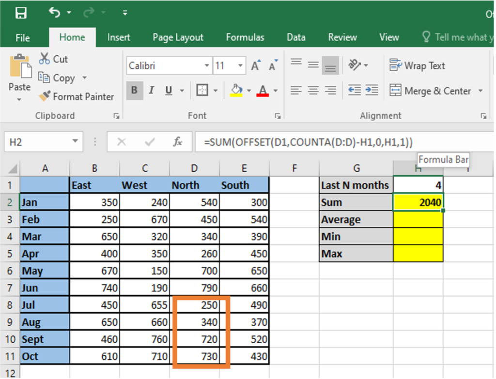
In the same way as we have used the SUM function with offset function, we can use other functions like average, min, and max functions with offset function. Suppose in the above example two more months i.e., September and October are added, and we want to know the sum, average, min and max values for the N months (Jul, Aug, Sep, Oct). We will use the below syntax for each case.

Sum of N months: =SUM(OFFSET(D1,COUNTA(D:D)-H1,0,H1,1))

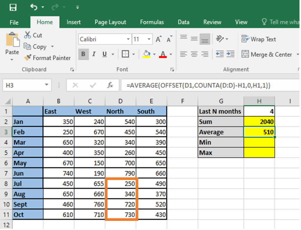
Average for N months: =AVERAGE(OFFSET(D1,COUNTA(D:D)-H1,0,H1,1))

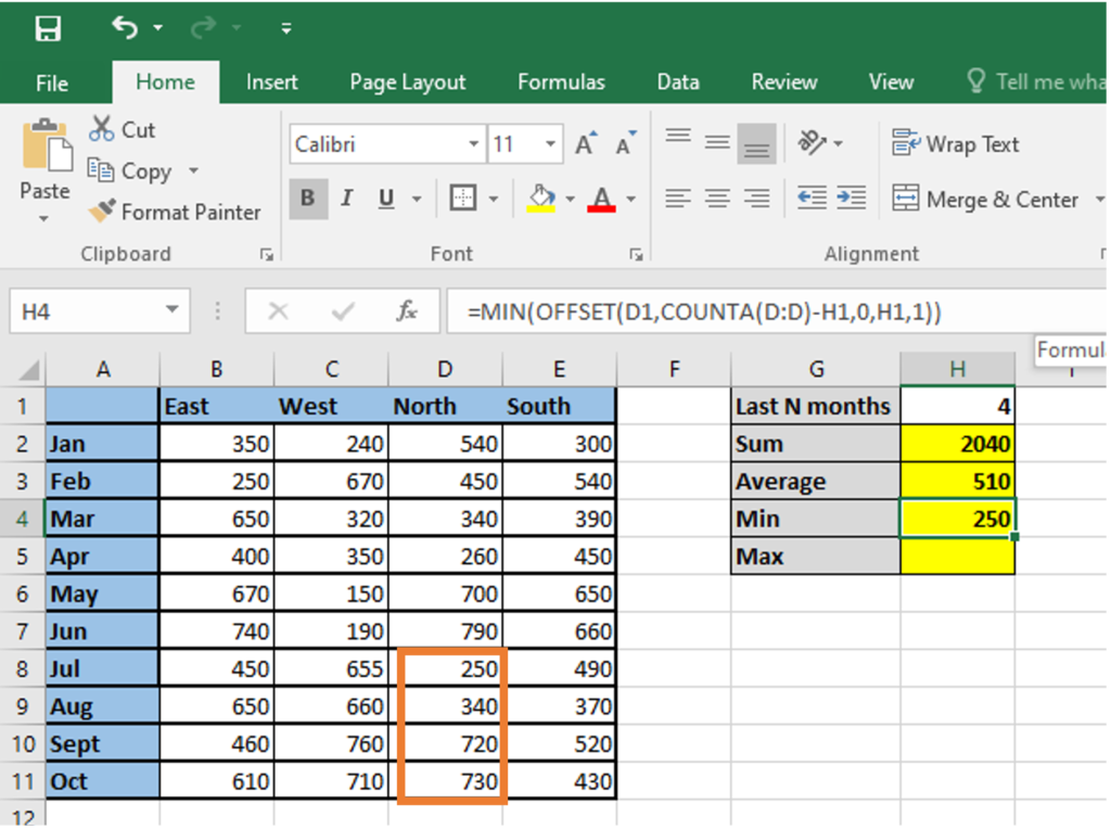
Min for N months: =MIN(OFFSET(D1,COUNTA(D:D)-H1,0,H1,1))

Max for N months: =MAX(OFFSET(D1,COUNTA(D:D)-H1,0,H1,1))

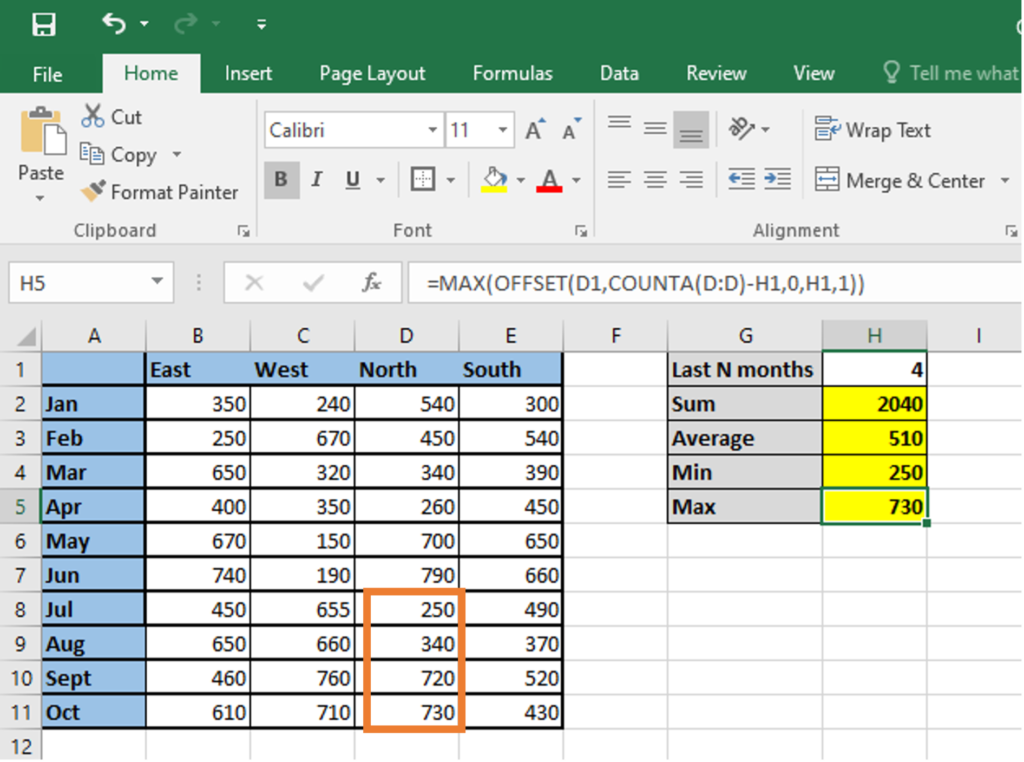
The most important benefit of using the offset function along with the regular average function is that there is no need to manually update the formula every time a new row is added to the table above, and the formula will auto calculate the sum, average, min or max of the lower most N number of cells mentioned in the formula.

CREATING DYNAMIC DROPDOWN LIST USING THE EXCEL OFFSET FUNCTION

We can create a dynamic dropdown list if the list being used is being regularly updated using the Offset function. This list is updated automatically whenever a new item is added or removed from the list.

Suppose we want to create a dynamic list of month name and want it to be automated so that whenever a new month is added to the worksheet, it gets updated in the dropdown list too.

The following steps can be followed to create such a dynamic list:

1. We can create a dynamic named range for the list of months using the offset function. We need to first write down the formula in any cell of the worksheet to create a dynamic named range. The syntax for the same shall be

=OFFSET(‘Region wise sales’!$A$1,0,0,COUNTA(‘Region wise sales’!$A:$A),1)

Where,                                                                                    

• Region_wise_sales: is the sheet name where the range is present
• A: is the column where the drop-down items are present
• $A$2: the cell containing the first item of the range

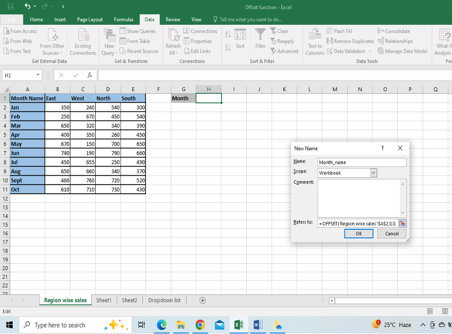
• Next we will copy this syntax and press Ctrl+F3 to open the New Name dialog box. We will enter the name for the range in the Name box (here it is named as : Month_name) and in the Refers to box we shall enter the Offset formula typed in step1 and enter OK.

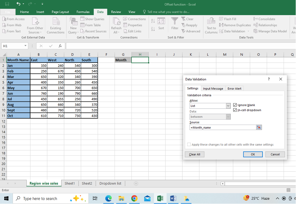
• Next we have to create a drop down list in any cell of the worksheet. Suppose we want to create a drop down list in cell H2 of Region_wise_sales sheet, we will go to the Data tab and select Data validation. In the setting tab therein under the allow box select the option named list and in the source tab enter the named range created in step2 as =Month_name.

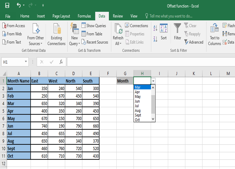
• We will get the dynamic dropdown list as below

 If we add the month Nov, the list will automatically show the new month Nov as below

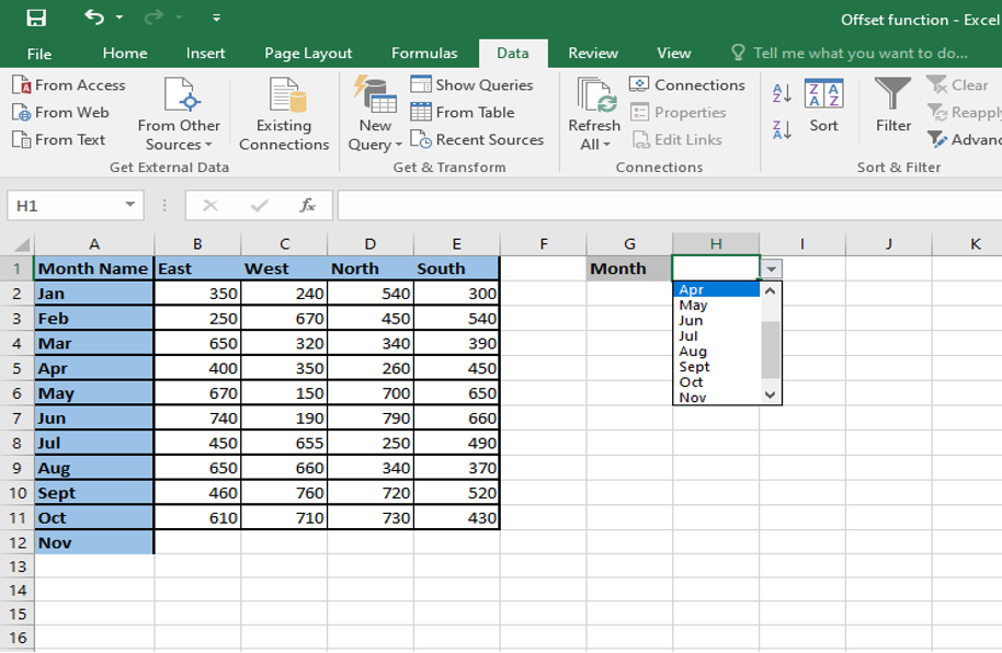
In this entire process the COUNTA function counts the non-blank cells in the specified column and the offset function uses this COUNTA as the height argument so that it returns a reference to a range that includes only non-empty cells starting from the first cell specified in the reference argument. The advantage to this process is that the dropdown list gets updated automatically without having to change the range selected for the drop down list.

Conclusion: As you can see from the above illustrations, Excel Offset function is a really handy tool to undertake dynamic calculations in Excel. The interactivity of your Excel data workbook dramatically improves the user experience to undertake data analysis in a very dynamic way.