A Leveraged Buyout – LBO financial model is a fundamental tool for private equity investors, providing a powerful framework to evaluate the feasibility of acquiring a company using a mix of debt and equity. LBO modeling helps assess the potential returns from such transactions, where a significant portion of the purchase price is financed through debt, making it a unique and highly leveraged form of acquisition. By leveraging borrowed funds, LBOs amplify returns and create significant value through careful planning and financial engineering. While this compelling investment strategy may seem complex, a well-designed LBO financial model simplifies the process by assessing profitability and risk. To bring these concepts to life, we will explore the fundamentals of LBO modeling through the lens of a retail company example, showcasing how industry-specific insights shape financial decision-making.
WHAT IS A LBO FINANCIAL MODEL?
A leveraged buyout is a strategic acquisition where a company is purchased primarily using debt, with the acquired company’s assets often serving as collateral. The goal is to generate sufficient cash flow to repay the debt while providing substantial returns to equity investors upon exit, typically through a sale or public offering.
An LBO financial model simulates the entire lifecycle of this acquisition, from the initial funding structure to the final exit. It helps investors assess whether the target company can support the debt while delivering attractive returns.
CORE ELEMENTS OF A LBO FINANCIAL MODEL
A LBO financial model calculates the potential returns from acquiring a target company, where a substantial portion of the purchase price is financed through debt. This strategic use of leverage allows private equity firms to amplify returns while minimizing their equity investment.
Post-acquisition, the private equity sponsor typically manages the company for 5–7 years, relying on the company’s free cash flows (FCFs) to reduce debt annually. This approach not only decreases financial risk but also enhances the equity value by the time of exit.
Hence, to understand the above we will study in detail the following core components of a LBO financial model.
- Entry Valuation
- Source and Uses of Invested Funds
- Financial Projections
- Debt Schedule
- Cash Flow Analysis
- Exit Valuation
- LBO Return Metrics like IRR
STEP-BY-STEP GUIDE TO MODELING A LBO FINANCIAL MODEL
Creating a Leveraged Buyout (LBO) financial model involves meticulous planning and detailed analysis to evaluate the potential profitability of acquiring a company using debt. Below are the key steps involved in building an LBO financial model, broken down for clarity:
STEP 1: BUILD THE TRANSACTION ASSUMPTIONS
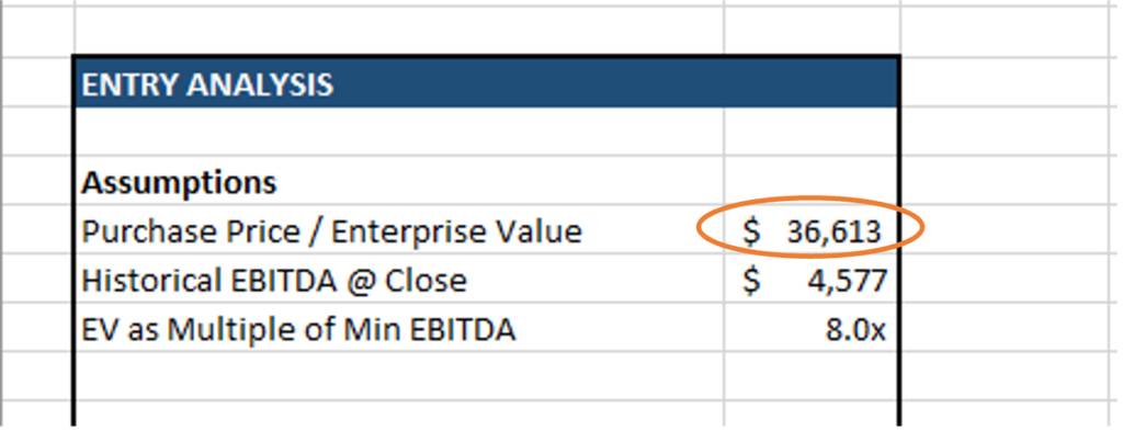
When building an LBO financial model, the first step is to do an entry valuation and establish the deal structure and financing requirements. The purchase price, calculated using an entry multiple like Enterprise Value (EV) to EBITDA multiple, serves as the foundation. For example, with an 8.0x multiple applied to the target company’s historical EBITDA of $4,577 million, the total purchase price, or EV, is determined to be $36,613 million.
See below how we have shown the Entry Valuation in our LBO financial model.
STEP 2: DETERMINING THE SOURCES AND USES OF FUNDS
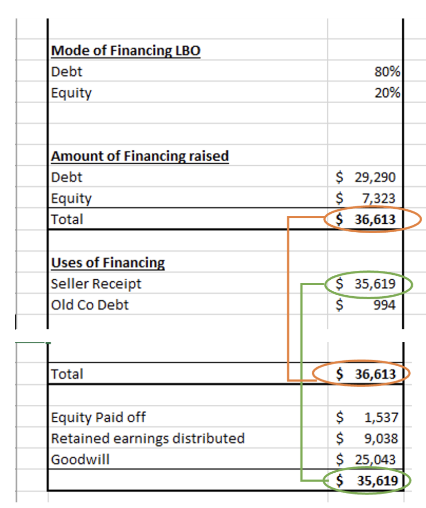
The next step involves detailing the sources of funds including equity, senior debt, mezzanine debt, or any other financing instruments. In this case, 80% of the financing, or $29,290 million, is funded through debt, while the remaining 20%, equivalent to $7,323 million, is raised as equity. This combination of debt and equity highlights the leveraged structure of the buyout.
The uses of funds must align perfectly with the sources of funds. Here, $35,619 million is allocated to the seller as part of the purchase consideration, while $994 million is used to repay the company’s existing debt. The allocation aligns perfectly, ensuring the total purchase price of $36,613 million is covered. Additional breakdowns include equity payouts of $1,537 million, distributed retained earnings of $9,038 million, and goodwill valued at $25,043 million, all critical components that highlight how the transaction is structured and financed.
This structured approach ensures all financing aspects of the LBO are mapped clearly, setting the stage for evaluating returns and profitability.
Let’s see below how we have shown the Entry Valuation in our LBO financial model.
Download our LBO financial model to understand the LBO-related adjustments and forecast your own LBO transaction.
STEP 3: CREATE THE OPERATING MODEL
The next step in building an LBO financial model is creating a detailed operating model to project the financial performance of the target company. Start by forecasting revenue, using historical growth rates, market trends, or industry-specific drivers to estimate future sales. Then, incorporate operating costs such as cost of goods sold (COGS), SG&A expenses, and other expenses to calculate EBITDA, a key measure of profitability. Additionally, factor in capital expenditures (CapEx) to account for investments required for growth or maintenance of assets. Lastly, include changes in working capital, such as fluctuations in receivables, payables, and inventory, to understand their impact on cash flow. Together, these elements create a comprehensive view of the company’s operating performance, enabling a more accurate assessment of its ability to service debt and generate returns.
In our model, all assumptions regarding the growth and projection of revenue, cost of goods sold, SG&A, Capex, Depreciation, and Interest Income are given in the Schedules sheet of Excel.
STEP 4: DESIGN THE DEBT SCHEDULE
A carefully structured debt schedule is critical in an LBO model, as it determines the allocation of cash flows and the timeline for debt repayment. Referring to the table above, the acquirer inherits the existing debt of $994 at the LBO transaction date in December 2024, with repayment contingent on a positive cash balance in the cash flow statement. This prudent approach ensures that the company maintains sufficient liquidity to manage its operations effectively.
The debt schedule captures the addition of $29,290 in new debt as part of the LBO financing in December 2024. The beginning debt balance rises sharply to reflect this leveraged structure. Starting in 2025, annual debt repayments of $5,000 are modeled, reducing the ending balance incrementally each year. Interest payments, calculated at 4% post-LBO, are directly linked to the outstanding debt balance of the previous year and decline as the debt is paid down.
This detailed schedule provides a comprehensive view of how debt obligations are managed over time, balancing aggressive repayments with the need to sustain positive cash flows and support operational requirements. By the end of 2029, the outstanding debt is projected to be reduced significantly to $4,290, demonstrating effective utilization of cash flow for deleveraging.
Let’s see below the debt schedule we have created in our LBO financial model.

STEP 5: FORECAST THE INCOME STATEMENT
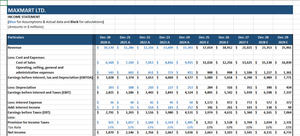
Forecasting the income statement is crucial in an LBO transaction as it provides a clear view of the company’s future profitability and cash flow, critical for assessing debt repayment capacity and investor returns. For Maxmart Ltd., revenue projections growing from $10,130 million in 2020 to $25,961 million in 2029, along with calculated costs and EBITDA growth, highlight the company’s operational efficiency. The forecast also considers the impact of the LBO’s leveraged structure, reflected in rising interest expenses and gradual repayment of debt, ensuring accurate net income projections. This step is vital for determining the deal’s feasibility and financial sustainability.
Below is the Income Statement projected for the LBO financial model.
STEP 6: BUILD THE BALANCE SHEET
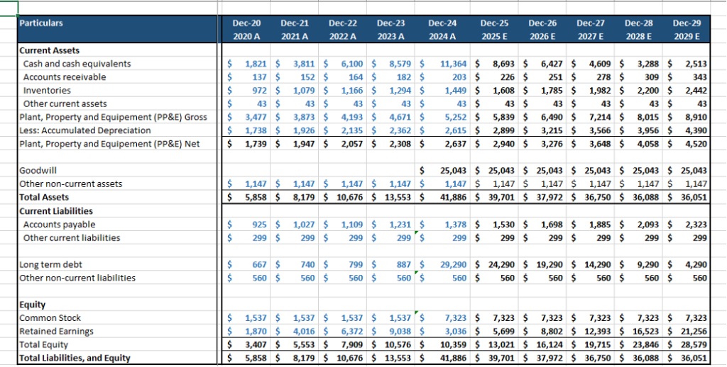
Building the balance sheet in an LBO financial model is crucial as it consolidates the financial structure post-buyout, ensuring the assets are appropriately financed by a mix of debt and equity. After forecasting the income statement and cash flow statement, the balance sheet reflects how the company’s profitability and cash generation impact key financial elements like debt repayment, working capital, and retained earnings. For instance, Maxmart Ltd.’s long-term debt of $29,290 million in 2024 gradually decreases, showcasing the model’s focus on deleveraging. Similarly, rising retained earnings signal profitability and equity growth. This step ensures the financial model remains balanced and provides a clear picture of the company’s leverage ratios and financial stability throughout the transaction.
Below is the Balance Sheet of our financial model.
STEP 7: BUILD THE CASH FLOWS STATEMENT
The cash flows statement serves as the bridge connecting the operating model to the debt schedule, offering a comprehensive view of how cash moves through the business. It begins with operating cash flow, which is derived from Net Income from the Income Statement, plus all non-cash expenses like depreciation and amortization, changes in working capital, and other operational factors. Next comes investing cash flow, where capital expenditures (CapEx), purchase of business through LBO, and potential acquisitions are deducted, reflecting the company’s long-term investment strategy. Finally, the financing cash flow accounts for debt repayments and any equity distributions, ensuring these commitments are accurately captured or funds raised through debt and equity.
The resulting cash flow reveals whether the company can comfortably meet its debt obligations while still generating returns for investors. This critical analysis highlights the sustainability of the leveraged structure and offers insights into the company’s financial health and capacity to create value over time.
Let’s see the Cash Flow Statement of our Financial Model below.
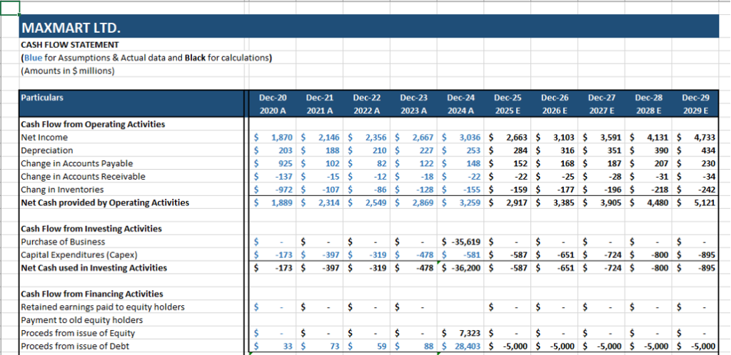

From the above Cash Flow Statement, we can see that the company generates most of the cash from operating activities as a result of improved operations. The company uses this operating cash flow to gradually repay its debt taken as a part of the LBO transaction.
STEP 8: MODEL THE EXIT ASSUMPTIONS
The exit analysis section of an LBO model focuses on calculating the implied valuation of the company at the time of exit, often based on an EBITDA multiple. In this example, the EBITDA multiple is set at 8.0x (same as the entry multiple), a key metric used to estimate the company’s enterprise value. As of December 2029, the target company has an EBITDA of $7,771 mn, which is multiplied by the exit multiple of 8.0x, yielding an enterprise value of $62,164 mn.
To determine the equity value, we subtract the company’s debt of $4,290 mn and add cash reserves of $2,513 mn as of December 2029, which results in an equity value of $60,387 mn by the end of 2029. This calculation reflects the value that the acquirer can potentially realize from the leveraged buyout, providing a clear picture of the expected return at the time of exit.
EQUITY VALUE = ENTERPRISE VALUE – DEBT + CASH
See below how the Exit valuation is done in our LBO financial model.

STEP 9: CALCULATE KEY OUTPUTS AND METRICS
Key metrics play a crucial role in assessing the investment’s performance, offering meaningful insights into its financial stability and growth prospects. The Internal Rate of Return (IRR), a critical measure of the investment’s annualized return, is calculated at 52%, demonstrating strong returns on the equity investment. IRR is calculated by taking the Equity value at the beginning and end of the LBO period as below:

The Debt Metrics give a detailed picture of the company’s leverage and financial stability. Total debt begins at $667 in December 2020 and climbs significantly to $29,290 by the end of 2024 due to the leveraged buyout, before gradually decreasing to $4,290 by 2029. The Debt-to-Equity ratio, which measures the level of debt relative to equity, peaks at a concerning 2.83 in 2024 due to a leveraged buyout but improves dramatically over the next few years, reaching 0.15 by 2029, reflecting a reduction in financial risk as debt is paid down.
Furthermore, the Interest Coverage Ratio, which indicates the company’s ability to cover interest payments with its operating income, starts at an impressive 79 in 2020 and stays robust until the buyout in 2025, where it drops to 4 but gradually increases to 20 by 2029, signaling a steady recovery in the company’s financial position.

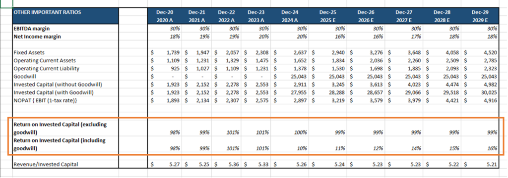
Return on Invested Capital (ROIC) excluding goodwill remains strong, ranging from 98% to 100% from 2020 to 2024, highlighting the company’s efficient use of capital in generating returns. We can see that after factoring in goodwill, the ROIC drops to 10% in the year 2024 from 101% in 2023, which however grows up to 16% by the year 2029. These metrics provide a comprehensive overview of the investment’s performance, helping guide future decision-making and illustrating the path toward a successful exit strategy.
STEP 10: PERFORM SENSITIVITY ANALYSIS
To truly assess the strength of an LBO model, it’s essential to conduct sensitivity and scenario analysis, testing the model’s resilience under varying assumptions. By adjusting the revenue growth rates, we can examine how changes in business performance directly impact cash flow and the company’s debt capacity. A shift in growth projections can significantly alter the company’s ability to service debt, making this a critical factor in understanding both risks and opportunities.
Furthermore, altering the entry and exit multiples allows us to explore different exit valuation scenarios, revealing how changes in the company’s valuation at the time of sale can affect equity returns. The sensitivity table provides a clear illustration of this, showing how different exit multiples (ranging from 6x to 10x) impact equity returns at varying entry multiples (6x to 10x). For example, at an entry multiple of 6x, and an exit multiple of 8x, IRR would be 66%, while at a higher exit multiple of 12x, the return jumps to 79%.
Lastly, evaluating how varying debt levels affect the deal’s feasibility is key. Increasing leverage can magnify returns, but it also raises risk, while reducing debt lowers risk but might limit the upside. By analyzing these different scenarios, the model’s robustness is tested, helping investors make more informed decisions about the potential risks and rewards of the LBO.
Let’s see below the sensitivity table we have built in our financial model.
- Sensitivity of IRR w.r.t Entry and Exit Multiple

In the above table, we are taking first input as entry multiple and the second input as exit multiple to get the sensitivity of IRR.
WHY LBO FINANCIAL MODELS MATTER?
An LBO financial model is more than a spreadsheet; it’s a decision-making framework that ensures investors understand the risks and rewards of a deal. By balancing leverage, cash flow, and exit opportunities, it provides a roadmap for creating value while managing financial risk.
CONCLUSION
Mastering the basics of an LBO financial model unlocks opportunities to transform undervalued companies into high-performing assets. Whether you’re an investor, analyst, or finance enthusiast, understanding how these models work is essential for navigating the dynamic world of private equity. With a clear grasp of the fundamentals, the complexity of leveraged buyouts becomes an exciting challenge rather than a daunting task.


