In corporate finance, predicting financial outcomes is crucial for making smart business decisions and planning ahead. Among the various forecasting methodologies, bottom-up forecasting stands out for its precision and practicality. By building forecasts from granular, operational data, this approach provides a clear and actionable roadmap for companies, ensuring that projections align closely with real-world conditions.
WHAT IS BOTTOM-UP FORECASTING?
Bottom-up forecasting involves estimating financial performance by aggregating detailed, component-level data. Rather than relying on broad assumptions, this approach starts with specific metrics like store-level sales, total retail area or employee headcount, or unit-level costs. These micro-level inputs are then combined to project revenue, expenses, and profitability at the organizational level.
For instance, a retail giant like Walmart might project its Total Store Revenue by calculating Average Revenue per square feet (No. of transactions per square feet * Transaction value) and multiplying it with the Total Retail Area (Sq feet) in the forecast period. Similarly, operating expenses such as rent, utilities, and labour are calculated for individual stores and then scaled up.
KEY STEPS IN BOTTOM-UP FORECASTING
- Identify Key Drivers: Determine the operational metrics that directly influence financial performance. For a retail company, these might include store count, average sales per store, and online sales growth.
- Collect Accurate Data: Use historical data and industry benchmarks to inform assumptions. For example, average annual salary per employee or rent per square foot or store can serve as reliable inputs.
- Build Segment-Level Forecasts: Calculate revenue and costs for each segment (e.g., physical stores, e-commerce). Segment-level granularity ensures that unique dynamics, such as differing growth rates for online and in-store sales, are captured.
- Aggregate to Financial Statements: Combine the forecasts for all segments to create income statements, balance sheets, and cash flow statements. Incorporate common expense categories like cost of goods sold (COGS), SG&A expenses, and corporate overheads.
FORMULA FOR BOTTOM UP FORECASTING OF REVENUE
The formula for bottom-up forecasting of revenue depends on the level of granularity and the nature of the business. A typical approach is to calculate revenue at a granular level and aggregate it to a company-wide total. The general formula is:
REVENUE = (QUANTITY OR UNIT VOLUME) × (PRICE PER UNIT)
EXAMPLE OF A FINANCIAL MODEL BASED ON BOTTOM-UP FORECASTING APPROACH
We can explain the methodology to model financial statements based on bottom up approach using a hypothetical example of a retail company named Maxmart Ltd. The foremost item to be forecasted is the revenue. We first need to identify the key revenue drivers from the financial statements or annual report of the company. In the retail company the common revenue drivers are Revenue per square foot, Order frequency and average order value. You can download the template of a bottom-up forecasting financial model for you to be able to practice on your own as well.
FORECASTING INCOME STATEMENT LINE ITEMS IN A FINANCIAL MODEL
1. Forecasting Revenue
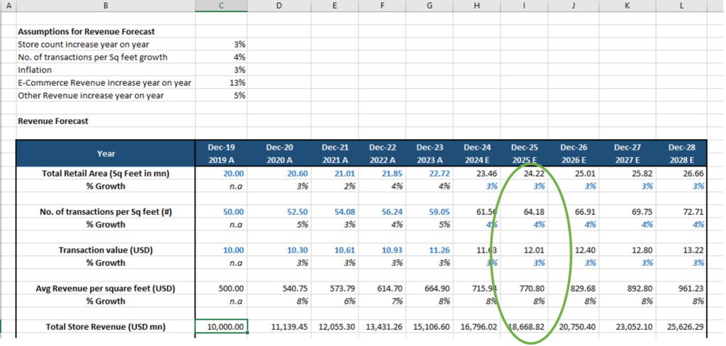
In our example we will be calculating Total Store Revenue using bottom up approach and the key drivers being Total Retail Area (square feet in mn) and Average Revenue per square feet (No. of transactions per square feet * transaction value).
Assumptions: We have taken the actual financial figures from the year 2019 to 2023 and based on the historical figures we will forecast the future financial statements using bottom up approach. We have assumed that the store count increases y-o-y by 3% (average growth of last 5 years), no. of transactions per square feet growth as 4% (average growth of last 5 years) and Inflation as 3%. Based on the above assumptions we have forecasted the revenue as below:
Total Store Revenue (USD mn) = Total Retail Area ( Square feet in mn) * No. of Transactions per Square feet(#) * Transaction value (USD)
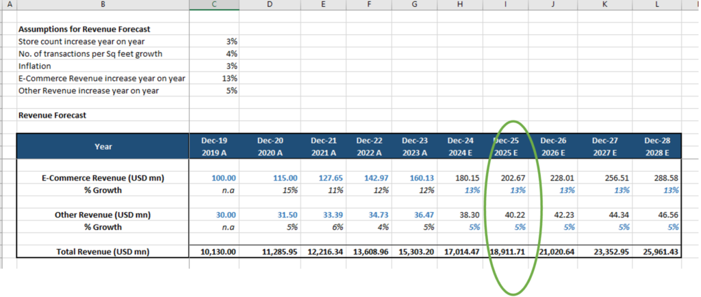
The retail company in our example also generates e-commerce revenue and revenue from other sources. Instead of Bottom up approach we have forecasted the future e-commerce and other revenue at an average growth rate of last 5 years’ e-commerce and other revenue.
**
2. Forecasting Expenses – Cost of Sales
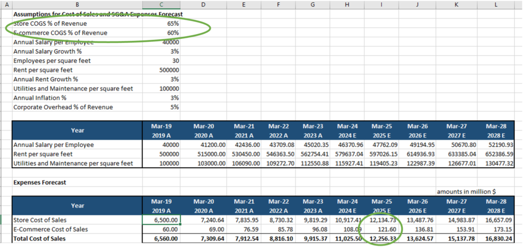
We will now forecast the expenses of the retail company in our example. The store cost of sales has been forecasted as a percentage of total store revenue and e-commerce cost of sales have been forecasted as a percentage of e-commerce revenue year on year.
Assumptions: Store cost of sales as a percentage of total store revenue is assumed to be 65% and e-commerce cost of sales as a percentage of e-commerce sales is assumed to be 60% based on the average percentage of the last 5 years each for store cost of sales and e-commerce cost of sales. Let’s see how it is calculated for the year 2025.
Store cost of sales (2025) = Total Store revenue (2025) * 65%
= $18,668.82 mn * 65%
= $ 12,134.73 mn
E-Commerce cost of sales (2025) = E-Commerce sales (2025) * 60%
= $202.67 mn * 60%
= $121.60 mn
**
3. Forecasting SG&A Expenses – Labour, Rent, Utilities, Marketing, Overheads
We can calculate the labour costs, rent expenses and utilities and maintenance expenses using the bottom up approach to forecast the SG&A expenses of the business.
The key driver for labour costs is annual salary per employee and employees per square feet. While considering annual salary growth rate of 3% assumed on the basis of average growth rate of last 5 years the total labour cost can be calculated as below.
Labour costs (2025) = Annual salary per employee* Growth rate* Employees per square feet*Total retail area
= $40,000*(1+3%)^6*30*24.22 / 1000000 = $34.70 mn
The key driver for rent expenses is rent per square feet and total retail area. While considering annual rent growth rate of 3% assumed on the basis of average growth rate of last 5 years the total rent expenses can be calculated as below.
Rent expenses (2025) = Rent per square feet* Annual rent growth rate* Total retail area
= $500,000*(1+3%)^6* 24.22 / 1000000
= $14.46 mn
The key driver for utilities and maintenance expenses is utilities and maintenance expenses per square feet and total retail area. While considering annual inflation rate of 3% assumed on the basis of average annual inflation rate of last 5 years the total utilities and maintenance expenses can be calculated as below.
Utilities and Maintenance (2025) = Utilities and Maintenance per square feet * Annual Inflation rate * Total retail area
= $10,00,00*(1+3%)^6* 24.22 mn / 1000000
= $2.89 mn
However, Corporate overhead and marketing expenses is calculated as a percentage of revenue. The percentage is taken as 5% based on the average of last 5 years’ corporate overhead and marketing expenses as a percentage of revenue.
Corporate Overhead and Marketing (2025) = Total Revenue * 5%
= $18,911.71 mn *5%
= $945.59 mn
Let’s see the snap shot of expenses calculated for all the years below.
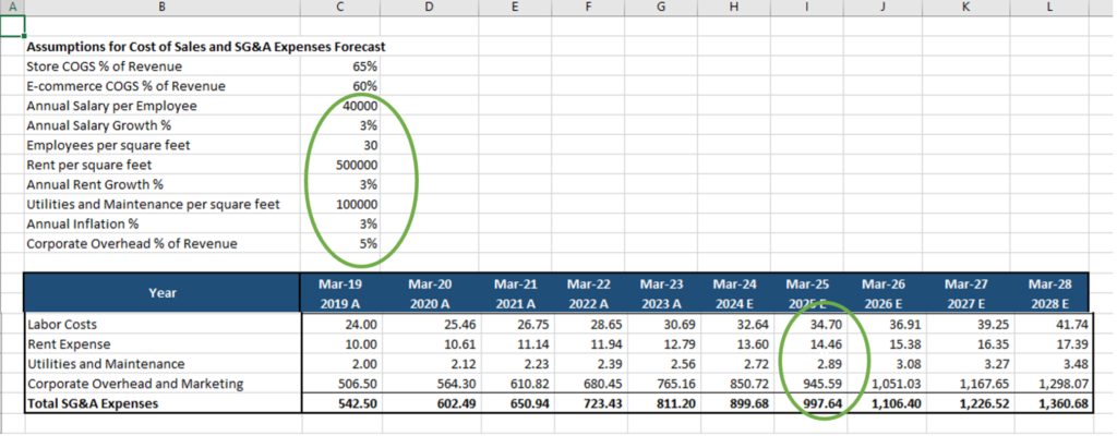
If we add up all the above expenses, the total SG&A expenses comes to $997.64 mn for FY 2025.
**
4. Forecasting Depreciation
In our financial model, we have calculated Depreciation on a straight line basis on the opening gross block of PP&E assuming the life of the asset to be around known.
Assumptions: The life of the asset is assumed to be 18.5 years and depreciation rate as 5.41% based on the average useful life and depreciation rate applied on gross block of fixed assets over the last 5 years. We have assumed in our model that the company maintains the asset productivity over the forecast period and hence we calculate Gross Block as a percentage of revenue (34%), which is the average gross block to revenue of the last 5 years.
The addition to PP&E, i.e, CAPEX is calculated as a difference between the Gross block and depreciation of the year.

**
5. Forecasting Interest Expenses & Interest Income
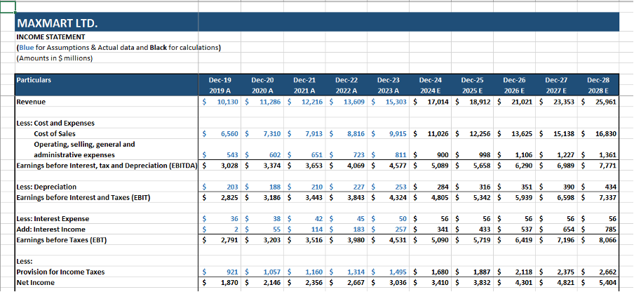
The interest expense is calculated for the forecast period at 5.65% on the closing balance of the loan for the previous year. The interest rate is assumed to be the average interest rate over the last 5 years. For example, in our example interest expense for the year 2025 is calculated on the closing balance of loan amount for 2024, which is $994 mn and multiplied with the average interest rate of 5.65%. Hence, interest expense is $56 mn.
The interest income is calculated for the forecast period at 3% on the closing balance of cash and cash equivalents of the previous year. The interest rate is assumed to be the average interest rate applied on cash and cash equivalents over the last 5 years. For example, in our example interest income for the year 2025 is calculated on the closing balance of cash and cash equivalents amount for 2024, which is $14,440 mn and multiplied with the average interest rate of 3%. Hence, interest expense is $433 mn.

**
6. Forecasting Income Taxes
The provision for Income Taxes for any given year during the forecast period is calculated at an average tax rate of 33% applied on Earnings before taxes over the last 5 years.

**
After having explained the assumptions behind the forecast of all major items of the income statement, let’s have a look at the overall snapshot of the Income Statement for the retail company in our example.
**
FORECASTING BALANCE SHEET LINE ITEMS IN A FINANCIAL MODEL
1. Forecasting Net Working Capital
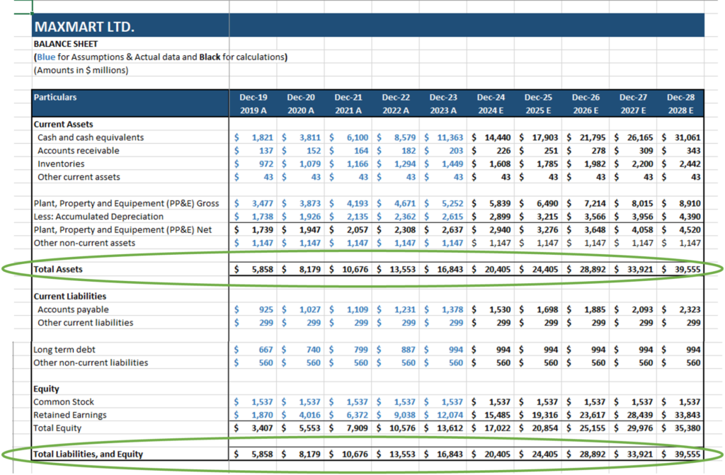
We have assumed that the company is maintaining its historical net working capital turnover (working capital as a % of Revenue). Hence, in our example for the forecasted period the Accounts Receivable is assumed to be at an average of last 5 years’ Accounts Receivable by Revenue ratio, Inventories is assumed at an average of last 5 years Inventories to Revenue ratio and Accounts Payable is kept at an average of last 5 years Accounts Payable to Revenue ratio year over year.
Other current assets and liabilities are assumed to be similar to the last historical year.

**
2. Forecasting Plant, Property and Equipment (PPE)
The basis for the forecast of plant, property and equipment (PP&E) gross amount is given above in the forecast of Income Statement items.
Assumptions: We have assumed in our model that the company maintains the asset productivity over the forecast period and hence we calculate Gross Block as a percentage of revenue (34%), which is the average gross block to revenue of the last 5 years.
The addition to PP&E, i.e, CAPEX is calculated as a difference between the Gross block and depreciation of the year.

The accumulated depreciation below PP&E gross in the balance sheet, is calculated as the depreciation for the year plus the depreciation for the previous fiscal years. PP&E net is hence the difference between the PP&E gross and accumulated depreciation.
3. Forecasting Debt
Long-term debt for the forecasted period of 5 years is assumed to be constant as the closing long-term debt balance at the end of year 2023. Hence, we are assuming that the company is not raising any new debt and not paying off the existing debt.
4. Forecasting Shareholders Equity
For the Equity we are assuming that the common stock amount remains constant as the company does not raise any further capital through issue of shares. We are also assuming that the company re-invests 100% of its net income into the growth of the company and hence retained earnings is calculated as the net income for any fiscal year plus net income for the previous fiscal years.
5. Forecasting Cash and Cash Equivalents
The cash and cash equivalents amount in the balance sheet for any fiscal year is linked with the ending cash and cash equivalents amount of the cash flow statement for that year.
**
After incorporating all the above assumptions, a snapshot of the Balance Sheet is presented below for reference. As you can notice, the total of the Assets side and the total of Liabilities & Equity is exactly same for all the years. This ensures our financial modeling linkages are correctly established in this exercise.
**
KEY REVENUE DRIVERS AND UNIT ECONOMICS ACROSS INDUSTRIES
| Industry | Quantity Drivers | Price Drivers |
| Retail (e.g., Walmart) | – Store count | – Product pricing |
| -Total square feet area | – Revenue per square feet | |
| – Units sold per store | – Discounting policies | |
| – Online order volumes | – Seasonal pricing variations | |
| SaaS (e.g., Salesforce) | – Customer acquisition rate | – Subscription pricing tiers (monthly/annual) |
| – Number of users or seats per customer | – Renewal rates | |
| – Customer churn rates | – Upselling and cross-selling prices | |
| Oil & Gas (e.g., ExxonMobil) | – Production volume (barrels of oil, gas output) | – Oil and gas prices (per barrel, per mcf) |
| – Refining throughput | – Regional pricing variations (e.g., Brent, WTI prices) | |
| Automotive (e.g., Ford) | – Vehicle production and sales volume | – Average selling price per vehicle |
| – Vehicle models (sedans, trucks, etc.) | – Pricing strategies for different models | |
| Telecommunications (e.g., Verizon) | – Number of subscribers (wireless, broadband) | – Data plans pricing |
| – Service usage (minutes, data consumed) | – Bundling options with other services (TV, internet) | |
| Healthcare (e.g., Hospital Networks) | – Patient visits or admissions | – Service charges for consultations, tests, and treatments |
| – Bed occupancy rate | – Insurance reimbursement rates | |
| Hospitality (e.g., Hotels) | – Room occupancy rate | – Room pricing (seasonal, peak pricing) |
| – Event bookings (weddings, conferences) | – Additional services (room service, spa services) pricing | |
| Consumer Goods (e.g., Procter & Gamble) | – Units sold per product category | – Price points based on product variants (premium vs. basic) |
| – Distribution channels (supermarkets, e-commerce) | – Promotional pricing (discounts, sales) |
HOW IS BOTTOM UP APPROACH DIFFERENT FROM TOP DOWN APPROCH OF FORECASTING FINANCIAL STATEMENTS
The top-down approach to forecasting financial statements focuses on macro-level data, such as industry trends, market size, and economic indicators, to project a company’s future performance. This method starts with broad assumptions, like the overall market size and a company’s market share, and works downward to estimate revenues, costs, and profits. For example, a company might estimate total revenue by calculating its share of a $1 trillion retail market rather than examining individual store sales. Costs and profits are then derived as percentages of revenue based on historical data or industry averages.
In contrast, the bottom-up approach builds forecasts from detailed, granular data, such as sales per store, labour costs, or rent. By aggregating these operational metrics, businesses can generate highly accurate and actionable projections. For example, a company like Walmart might calculate revenue by multiplying the average revenue per store by the number of stores and summing it with projected e-commerce sales.
Both approaches serve different purposes. Walmart might use the top-down approach for high-level strategic decisions, such as entering a new market or assessing overall industry trends. For instance, if the global retail market is expected to grow by 5%, Walmart could estimate its revenue growth based on its current market share. On the other hand, it might rely on the bottom-up approach for operational planning, such as budgeting store-level costs or forecasting employee wages. By combining these methods, Walmart can balance macro-level insights with operational precision, ensuring strategic alignment and accurate financial planning.
| Aspect | Top-Down Approach | Bottom-Up Approach |
| Starting Point | Begins with macro-level data (market size, GDP, etc.). | Starts with micro-level data (store-level sales, unit costs, etc.). |
| Data Granularity | Relies on broad assumptions. | Builds detailed, segment-specific forecasts. |
| Focus | External factors like market share and economic growth. | Internal operations, such as sales per unit or labour costs. |
| Complexity | Simpler and faster to implement. | More complex and time-intensive. |
| Accuracy | Less precise, especially for specific operational insights. | Highly accurate, as it accounts for granular factors. |
| Use Case | Useful for strategic planning and high-level projections. | Ideal for detailed budgeting and operational decision-making. |
PROS AND CONS OF THE BOTTOM-UP APPROACH FOR FORECASTING FINANCIAL STATEMENTS
| Pros | Cons |
| Provides highly accurate forecasts by starting with granular data (e.g., unit sales, costs). | Time-consuming due to the need for detailed data collection and processing. |
| Enables customization of assumptions, such as changes in wages, store count, or other variables. | Relies heavily on the accuracy and availability of granular data; poor inputs lead to errors. |
| Facilitates operational alignment by focusing on specific revenue and cost drivers. | Can overlook macroeconomic factors or broader industry trends if overly focused internally. |
| Supports scenario analysis to test multiple business strategies and conditions. | Complex and challenging to manage for large organizations with multiple components. |
| Reflects real-world operational conditions, enhancing reliability for decision-making. | Excessive detail can make the model rigid and less adaptable to unexpected changes. |
| Highlights areas for cost optimization and resource allocation improvements. | Resource-intensive, requiring significant manpower, time, and technological tools. |
CONCLUSION
Bottom-up forecasting offers a methodical approach to financial planning, providing businesses with detailed and actionable insights. Whether it’s a retail chain forecasting store revenues or a SaaS company estimating customer acquisition costs, this approach ensures accuracy and adaptability. By building financial statements from the ground up, businesses can navigate uncertainties with confidence and align their strategies with operational realities.
For companies aiming to enhance their financial planning, bottom-up forecasting isn’t just a methodology—it’s a pathway to clarity and control.


